35. Dimensionality Reduction#
Key takeaways
Use t-SNE or UMAP for ADT visualization; PCA can help reduce dimensionality in large datasets.
Environment setup
Install conda:
Before creating the environment, ensure that conda is installed on your system.
Save the yml content:
Copy the content from the yml tab into a file named
environment.yml.
Create the environment:
Open a terminal or command prompt.
Run the following command:
conda env create -f environment.yml
Activate the environment:
After the environment is created, activate it using:
conda activate <environment_name>
Replace
<environment_name>with the name specified in theenvironment.ymlfile. In the yml file it will look like this:name: <environment_name>
Verify the installation:
Check that the environment was created successfully by running:
conda env list
name: surface-protein
channels:
  - conda-forge
  - bioconda
dependencies:
  - scanpy=1.9.1
  - muon=0.1.5
  - harmonypy=0.0.9
  - glob2
  - leidenalg
  - numba>=0.56.4
  - pooch=1.7.0
35.1. Motivation#
Feature matrices of surface protein markers are hard to grasp for humans as raw tables. Therefore, we resort to low dimensional embeddings that allow us to visualize the ADTs in commonly two dimensions. The approaches that we use and recommend for ADT data do not differ from the ones for transcriptomics data. All aforementioned limitations of visualizations obtained through methods like t-SNE and UMAP also apply to ADT data.
ADT data generally does not require any sophisticated feature selection, because features have already been selected a priori during experimental design. All selected ADT should correspond to biologically relevant features. Nevertheless, large datasets may benefit from PCA to reduce the dataset from several hundred features to a couple of principal components. This is especially advisable if computational resources are limited.
35.2. Environment setup#
import muon as mu
import pooch
import scanpy as sc

# setting visualization parameters
sc.settings.verbosity = 0
sc.settings.set_figure_params(
    dpi=80,
    facecolor="white",
    frameon=False,
)
35.3. Loading the data#
cite_xdbt = pooch.retrieve(
    url="https://figshare.com/ndownloader/files/41452434",
    fname="cite_doublet_removal_xdbt.h5mu",
    path=".",
    known_hash=None,
    progressbar=True,
)
We are simply loading the saved MuData object from the normalization chapter back in.
mdata = mu.read("cite_doublet_removal_xdbt.h5mu")
As the isotypes do not contain any biological information, we can remove them from our data.
mdata["prot"].var.index[:50]
Index(['CD86-1', 'CD274-1', 'CD270', 'CD155', 'CD112', 'CD47-1', 'CD48-1',
       'CD40-1', 'CD154', 'CD52-1', 'CD3', 'CD8', 'CD56', 'CD19-1', 'CD33-1',
       'CD11c', 'HLA-A-B-C', 'CD45RA', 'CD123', 'CD7-1', 'CD105', 'CD49f',
       'CD194', 'CD4-1', 'CD44-1', 'CD14-1', 'CD16', 'CD25', 'CD45RO', 'CD279',
       'TIGIT-1', 'Mouse-IgG1', 'Mouse-IgG2a', 'Mouse-IgG2b', 'Rat-IgG2b',
       'CD20', 'CD335', 'CD31', 'Podoplanin', 'CD146', 'IgM', 'CD5-1', 'CD195',
       'CD32', 'CD196', 'CD185', 'CD103', 'CD69-1', 'CD62L', 'CD161'],
      dtype='object')
isotype_controls = ["Mouse-IgG1", "Mouse-IgG2a", "Mouse-IgG2b", "Rat-IgG2b"]
temp = mdata["prot"].var.loc[~mdata["prot"].var.index.isin(isotype_controls), :].index
temp
Index(['CD86-1', 'CD274-1', 'CD270', 'CD155', 'CD112', 'CD47-1', 'CD48-1',
       'CD40-1', 'CD154', 'CD52-1',
       ...
       'CD94', 'CD162', 'CD85j', 'CD23', 'CD328', 'HLA-E-1', 'CD82-1',
       'CD101-1', 'CD88', 'CD224'],
      dtype='object', length=136)
We store the isotype data as a multi-dimensional annotation.
mdata["prot"].obsm["X_isotypes"] = mdata["prot"].X[
    :, ~mdata["prot"].var.index.isin(temp.tolist())
]
mu.pp.filter_var(data=mdata["prot"], var=temp.tolist())
mdata["prot"].var.index[:50]
Index(['CD86-1', 'CD274-1', 'CD270', 'CD155', 'CD112', 'CD47-1', 'CD48-1',
       'CD40-1', 'CD154', 'CD52-1', 'CD3', 'CD8', 'CD56', 'CD19-1', 'CD33-1',
       'CD11c', 'HLA-A-B-C', 'CD45RA', 'CD123', 'CD7-1', 'CD105', 'CD49f',
       'CD194', 'CD4-1', 'CD44-1', 'CD14-1', 'CD16', 'CD25', 'CD45RO', 'CD279',
       'TIGIT-1', 'CD20', 'CD335', 'CD31', 'Podoplanin', 'CD146', 'IgM',
       'CD5-1', 'CD195', 'CD32', 'CD196', 'CD185', 'CD103', 'CD69-1', 'CD62L',
       'CD161', 'CD152', 'CD223', 'KLRG1-1', 'CD27-1'],
      dtype='object')
35.4. PCA and UMAP#
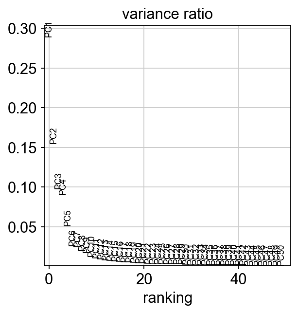
We can now reduce the dimensionality of the data with PCA since our dataset is very big, compute a neighborhood graph and a UMAP embedding to visualize the study’s variables.
sc.pp.pca(mdata["prot"], svd_solver="arpack")
sc.pl.pca_variance_ratio(mdata["prot"], n_pcs=50)
sc.pp.neighbors(mdata["prot"], n_pcs=20)
sc.tl.umap(mdata["prot"])
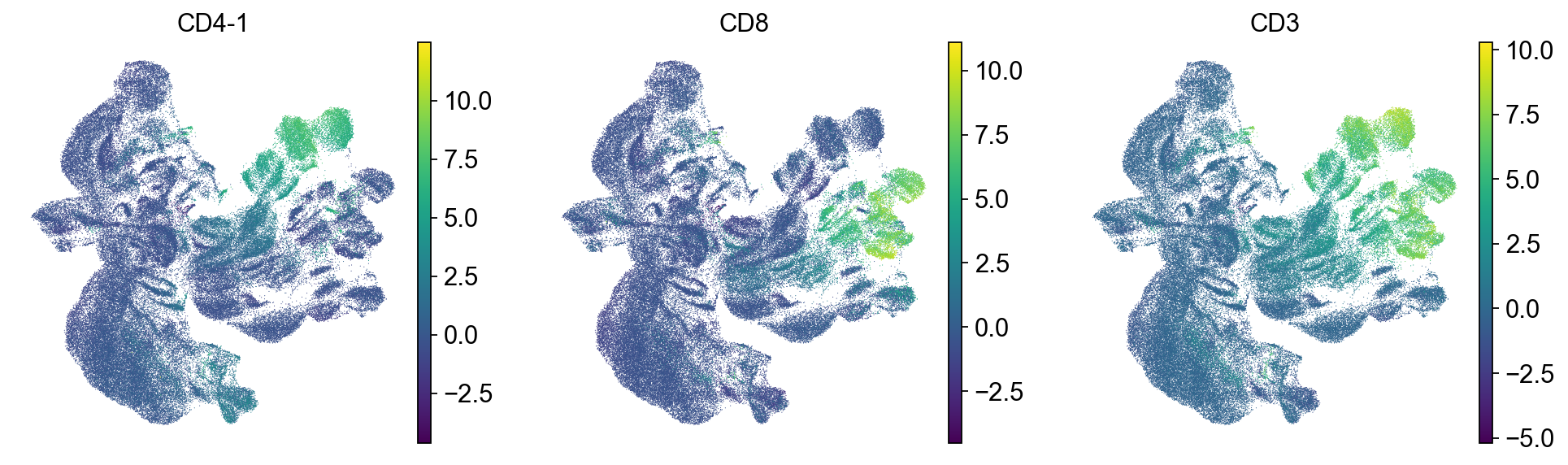
sc.pl.umap(mdata["prot"], color=["CD4-1", "CD8", "CD3"])
sc.pl.umap(mdata["prot"], color=["CD14-1", "CD16"])

sc.pl.umap(mdata["prot"], color=["donor", "batch"])
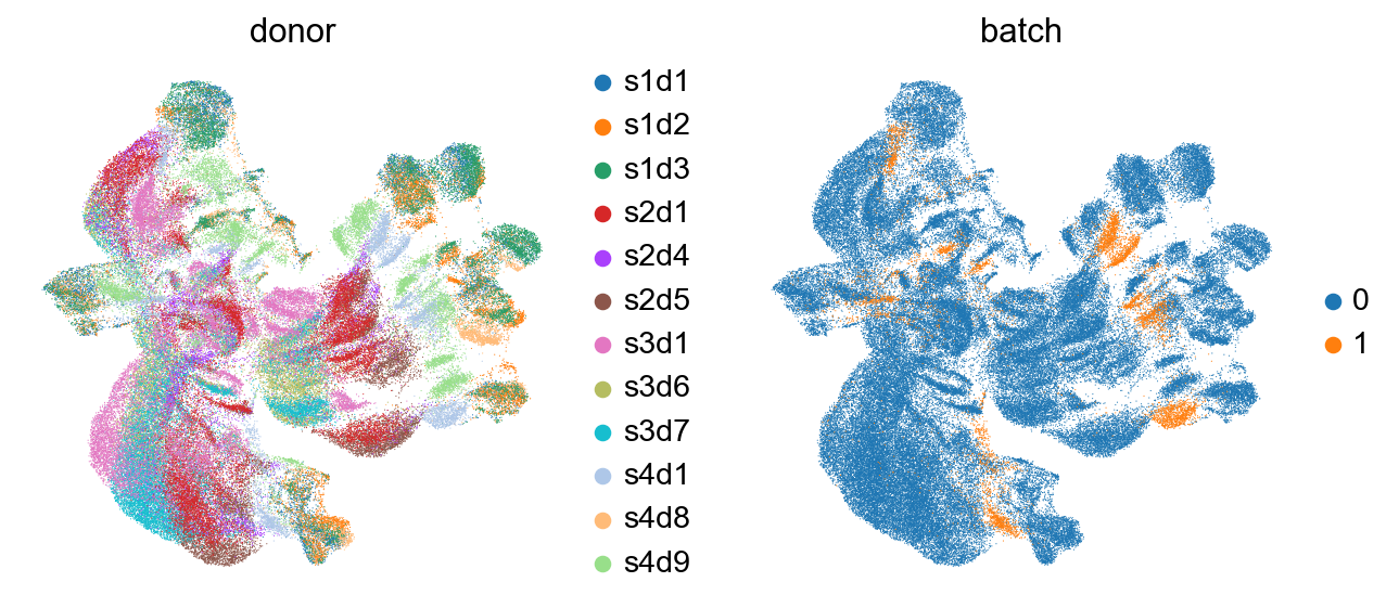
As it can be seen in the above UMAP representation, different samples cluster apart from each other for similar populations (see CD4 and CD8 expression in the previous plot). Thus, batch correction of the data would be necessary.
mdata
MuData object with n_obs × n_vars = 119837 × 36741
  var:	'gene_ids', 'feature_types'
  2 modalities
    rna:	119837 x 36601
      obs:	'donor', 'batch'
      var:	'gene_ids', 'feature_types'
    prot:	119837 x 136
      obs:	'donor', 'batch', 'n_genes_by_counts', 'log1p_n_genes_by_counts', 'total_counts', 'log1p_total_counts', 'n_counts', 'outliers', 'doublets_markers'
      var:	'gene_ids', 'feature_types', 'n_cells_by_counts', 'mean_counts', 'log1p_mean_counts', 'pct_dropout_by_counts', 'total_counts', 'log1p_total_counts'
      uns:	'doublets_markers_colors', 'pca', 'neighbors', 'umap', 'donor_colors', 'batch_colors'
      obsm:	'X_isotypes', 'X_pca', 'X_umap'
      varm:	'PCs'
      layers:	'counts'
obsp: 'distances', 'connectivities'mdata.write("cite_dimensionality_reduction.h5mu")
35.5. References#
35.6. Contributors#
We gratefully acknowledge the contributions of:
35.6.2. Reviewers#
Lukas Heumos
Anna Schaar