⚙️ Environment setup
Install conda:
Before creating the environment, ensure that conda is installed on your system.
Save the yml content:
Copy the content from the yml tab into a file named
environment.yml.
Create the environment:
Open a terminal or command prompt.
Run the following command:
conda env create -f environment.yml
Activate the environment:
After the environment is created, activate it using:
conda activate <environment_name>Replace
<environment_name>with the name specified in theenvironment.ymlfile. In the yml file it will look like this:name: <environment_name>
Verify the installation:
Check that the environment was created successfully by running:
conda env list
name: preprocessing
channels:
  - bioconda
  - conda-forge
dependencies:
  - conda-forge::ipykernel=7.3.0
  - conda-forge::ipywidgets=8.1.9
  - conda-forge::leidenalg=0.12.0
  - conda-forge::numba=0.67.0
  - conda-forge::python=3.13.15
  - conda-forge::r-base=4.5.3
  - conda-forge::r-soupx=1.6.2
  - conda-forge::r-sctransform=0.4.3
  - conda-forge::r-glmpca=0.2.0
  - conda-forge::rpy2=3.6.8
  - conda-forge::scanpy=1.12.4
  - conda-forge::session-info=1.0.0
  - bioconda::anndata2ri=2.0.1
  - bioconda::bioconductor-scdblfinder=1.24.10
  - bioconda::bioconductor-scry=1.22.0
  - bioconda::bioconductor-scran=1.38.1
  - bioconda::bioconductor-glmgampoi=1.22.0
  - pip
  - pip:
      - lamindb==2.10.0
🗄️ Get data and notebooks
This book uses lamindb to store, share, and load datasets and notebooks using the theislab/sc-best-practices instance. We acknowledge free hosting from Lamin Labs.
Install lamindb
Install the lamindb Python package:
pip install lamindbOptionally create a lamin account
Sign up and log in following the instructions
Verify your setup
Run the
lamin connectcommand:
import lamindb as ln

ln.Artifact.connect("theislab/sc-best-practices").df()
You should now see up to 100 of the stored datasets.
Accessing datasets (Artifacts)
Search for the datasets on the Artifacts page
Load an Artifact and the corresponding object:
import lamindb as ln

af = ln.Artifact.connect("theislab/sc-best-practices").get(
    key="key_of_dataset", is_latest=True
)
obj = af.load()
The object is now accessible in memory and is ready for analysis. Adapt the
lamindb.Artifact.connect("theislab/sc-best-practices").get("SOMEIDXXXX")suffix to get respective versions.Accessing notebooks (Transforms)
Search for the notebook on the Transforms page
Load the notebook:
lamin load <notebook url>which will download the notebook to the current working directory. Analogously to
Artifacts, you can adapt the suffix ID to get older versions.
Motivation
We now have a normalized data representation that still preserves biological heterogeneity but with reduced technical sampling effects in gene expression. ScRNA-seq datasets usually contain up to 30,000 genes (depending on the organism) and so far we only removed genes that are not detected in at least 20 cells. However, many of the remaining genes are not informative and contain mostly zero counts. Therefore, a standard preprocessing pipeline involves the step of feature selection which aims to exclude uninformative genes which might not represent meaningful biological variation across samples.
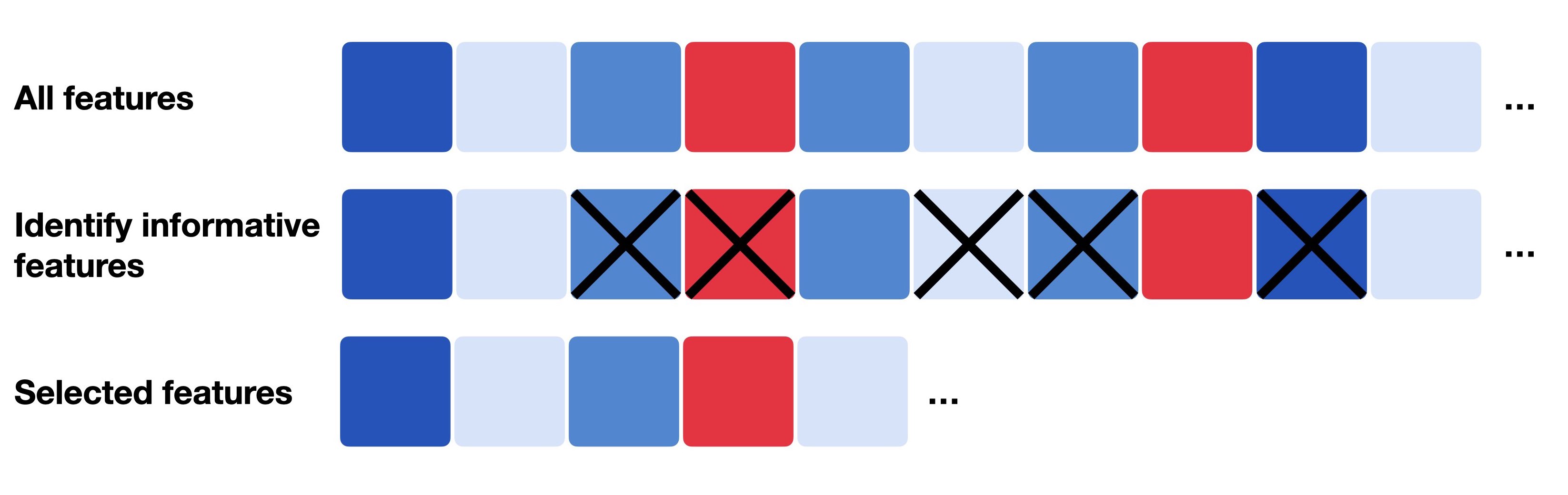
Figure 1:Feature selection generally describes the process of only selecting a subset of relevant features which can be the most informative, most variable or most deviant ones.
Often, the scRNA-seq experiment focuses on one specific tissue and hence, only a small fraction of genes is informative and biologically variable. Traditional approaches and pipelines either compute the coefficient of variation (highly variable genes) or the average expression level (highly expressed genes) of all genes to obtain 500-2000 selected genes and use these features for their downstream analysis steps. However, these methods are highly sensitive to the normalization technique used before. As mentioned earlier, a former preprocessing workflow included normalization with CPM and subsequent log transformation. But as log-transformation is not possible for exact zeros, analysts often add a small pseudo count, e.g., 1 (log1p), to all normalized counts before log transforming the data. Choosing the pseudo count, however, is arbitrary and can introduce biases to the transformed data. This arbitrariness has then also an effect on the feature selection as the observed variability depends on the chosen pseudo count. A small pseudo count value close to zero is increasing the variance of genes with zero counts Townes et al., 2019.
Germain et al. instead propose to use deviance for feature selection which works on raw counts Germain et al., 2020. Deviance can be computed in closed form and quantifies whether genes show constant expression profile across cells as these are not informative. Genes with constant expression are described by a multinomial null model, they are approximated by the binomial deviance. Highly informative genes across cells will have a high deviance value which indicates a poor fit by the null model (i.e., they don’t show constant expression across cells). According to the deviance values, the method then ranks all genes and obtains only highly deviant genes.
What does deviance measure?
Deviance is twice the gap in log likelihood between two models of a gene’s counts: one where every cell draws the gene at the same rate, and one that reproduces the counts exactly. Genes expressed at a constant rate are fit well by the shared rate and score low, while genes switched on in one population and off elsewhere score high.
Unlike variance, deviance is defined on raw counts, so it needs no normalization first and does not rank a gene highly just for being strongly expressed.
As mentioned before, deviance can be computed in closed form and is provided within the R package scry.
We start by setting up our environment.
import logging

import lamindb as ln
import matplotlib.pyplot as plt
import numpy as np
import rpy2.rinterface_lib.callbacks as rcb
import rpy2.robjects as ro
import rpy2.robjects.packages as rpackages
import scanpy as sc
import seaborn as sns
from rpy2.robjects import default_converter, numpy2ri, pandas2ri, r
from rpy2.robjects.conversion import localconverter

# Suppress verbose logging from Scanpy
sc.settings.verbosity = 0

# Set figure parameters for clean, minimal plots
sc.set_figure_params(dpi=80, facecolor="white", frameon=False)

rcb.logger.setLevel(logging.ERROR)

%load_ext rpy2.ipython

ln.connect("theislab/sc-best-practices")

ln.track("xKADqrV9wgwX")
Output
→ connected lamindb: theislab/sc-best-practices
→ loaded Transform('xKADqrV9wgwX0001', key='feature_selection.ipynb'), started new Run('FFyj7Rnk49KRDUdC') at 2026-09-29 11:57:52 UTC
→ notebook imports: lamindb-core==2.10.0 matplotlib==3.11.2 numpy==2.5.3 rpy2-rinterface==3.6.7 rpy2-robjects==3.6.5 scanpy==1.12.4 seaborn==0.13.2
• tip: to identify the notebook across renames, pass the uid: ln.track("xKADqrV9wgwX")
%%R
library(scry)
library(SingleCellExperiment)
Output
Loading required package: SummarizedExperiment
Loading required package: MatrixGenerics
Loading required package: matrixStats

Attaching package: ‘MatrixGenerics’

The following objects are masked from ‘package:matrixStats’:

    colAlls, colAnyNAs, colAnys, colAvgsPerRowSet, colCollapse,
    colCounts, colCummaxs, colCummins, colCumprods, colCumsums,
    colDiffs, colIQRDiffs, colIQRs, colLogSumExps, colMadDiffs,
    colMads, colMaxs, colMeans2, colMedians, colMins, colOrderStats,
    colProds, colQuantiles, colRanges, colRanks, colSdDiffs, colSds,
    colSums2, colTabulates, colVarDiffs, colVars, colWeightedMads,
    colWeightedMeans, colWeightedMedians, colWeightedSds,
    colWeightedVars, rowAlls, rowAnyNAs, rowAnys, rowAvgsPerColSet,
    rowCollapse, rowCounts, rowCummaxs, rowCummins, rowCumprods,
    rowCumsums, rowDiffs, rowIQRDiffs, rowIQRs, rowLogSumExps,
    rowMadDiffs, rowMads, rowMaxs, rowMeans2, rowMedians, rowMins,
    rowOrderStats, rowProds, rowQuantiles, rowRanges, rowRanks,
    rowSdDiffs, rowSds, rowSums2, rowTabulates, rowVarDiffs, rowVars,
    rowWeightedMads, rowWeightedMeans, rowWeightedMedians,
    rowWeightedSds, rowWeightedVars

Loading required package: GenomicRanges
Loading required package: stats4
Loading required package: BiocGenerics
Loading required package: generics

Attaching package: ‘generics’

The following objects are masked from ‘package:base’:

    as.difftime, as.factor, as.ordered, intersect, is.element, setdiff,
    setequal, union


Attaching package: ‘BiocGenerics’

The following objects are masked from ‘package:stats’:

    IQR, mad, sd, var, xtabs

The following objects are masked from ‘package:base’:

    anyDuplicated, aperm, append, as.data.frame, basename, cbind,
    colnames, dirname, do.call, duplicated, eval, evalq, Filter, Find,
    get, grep, grepl, is.unsorted, lapply, Map, mapply, match, mget,
    order, paste, pmax, pmax.int, pmin, pmin.int, Position, rank,
    rbind, Reduce, rownames, sapply, saveRDS, table, tapply, unique,
    unsplit, which.max, which.min

Loading required package: S4Vectors

Attaching package: ‘S4Vectors’

The following object is masked from ‘package:utils’:

    findMatches

The following objects are masked from ‘package:base’:

    expand.grid, I, unname

Loading required package: IRanges
Loading required package: Seqinfo
Loading required package: Biobase
Welcome to Bioconductor

    Vignettes contain introductory material; view with
    'browseVignettes()'. To cite Bioconductor, see
    'citation("Biobase")', and for packages 'citation("pkgname")'.


Attaching package: ‘Biobase’

The following object is masked from ‘package:MatrixGenerics’:

    rowMedians

The following objects are masked from ‘package:matrixStats’:

    anyMissing, rowMedians
Next, we load the already normalized dataset from the previous chapter.
Deviance works on raw counts so there is no need to replace adata.X with one of the normalized layers, but we can directly use the object as it was stored in the normalization notebook.
af = ln.Artifact.connect("theislab/sc-best-practices").get(
    key="preprocessing_visualization/s4d8_normalization.h5ad", is_latest=True
)
adata = af.load()
adata
AnnData object with n_obs × n_vars = 15998 × 20362
obs: 'n_genes_by_counts', 'log1p_n_genes_by_counts', 'total_counts', 'log1p_total_counts', 'pct_counts_in_top_20_genes', 'total_counts_mt', 'log1p_total_counts_mt', 'pct_counts_mt', 'total_counts_ribo', 'log1p_total_counts_ribo', 'pct_counts_ribo', 'total_counts_hb', 'log1p_total_counts_hb', 'pct_counts_hb', 'logit_mt_fraction', 'outlier', 'mt_outlier', 'soupx_groups', 'scDblFinder_score', 'scDblFinder_class', 'size_factors'
var: 'gene_ids', 'feature_types', 'genome', 'interval', 'mt', 'ribo', 'hb', 'n_cells_by_counts', 'mean_counts', 'log1p_mean_counts', 'pct_dropout_by_counts', 'total_counts', 'log1p_total_counts', 'n_cells'
layers: 'analytic_pearson_residuals', 'counts', 'log1p_norm', 'scran_normalization', 'soupX_counts', None (.X)Similar to before, we save the AnnData object in our R environment.
X_sparse = adata.X.T.tocoo()

Matrix = rpackages.importr("Matrix")

with localconverter(ro.default_converter + pandas2ri.converter + numpy2ri.converter):
    ro.globalenv["obs"] = adata.obs
    ro.globalenv["var"] = adata.var

i, j = X_sparse.row, X_sparse.col
x = X_sparse.data

ro.globalenv["i"] = ro.IntVector((i + 1).tolist())  # R is 1-indexed
ro.globalenv["j"] = ro.IntVector((j + 1).tolist())
ro.globalenv["x"] = ro.FloatVector(x.tolist())

r("X <- sparseMatrix(i = i, j = j, x = x, dims = c({}, {}))".format(*X_sparse.shape))
We can now directly call feature selection with deviance on the non-normalized counts matrix and export the binomial deviance values as a vector.
Our dataset is a single sample, but for several batches, passing them to the batch argument of devianceFeatureSelection fits the null model within each batch, so that differences between batches do not make genes look deviant.
%%R
sce <- SingleCellExperiment(
  assays = list(X = X),
  colData = obs,
  rowData = var
)

sce <- devianceFeatureSelection(sce, assay = "X")
Output
with localconverter(default_converter + pandas2ri.converter + numpy2ri.converter):
    binomial_deviance = ro.r("rowData(sce)$binomial_deviance")
As a next step, we now sort the vector and select the top 4,000 highly deviant genes and save them as an additional column in .var as ‘highly_deviant’.
We additionally save the computed binomial deviance in case we want to sub-select a different number of highly variable genes afterwards.
idx = binomial_deviance.argsort()[-4000:]
mask = np.zeros(adata.var_names.shape, dtype=bool)
mask[idx] = True

adata.var["highly_deviant"] = mask
adata.var["binomial_deviance"] = binomial_deviance
Last, we visualise the feature selection results. We use a scanpy function to compute the mean and dispersion for each gene across all cells.
sc.pp.highly_variable_genes(adata, layer="scran_normalization")We inspect our results by plotting dispersion versus mean for the genes and color by ‘highly_deviant’.
ax = sns.scatterplot(
    data=adata.var, x="means", y="dispersions", hue="highly_deviant", s=5
)
ax.set_xlim(None, 1.5)
ax.set_ylim(None, 3)
plt.show()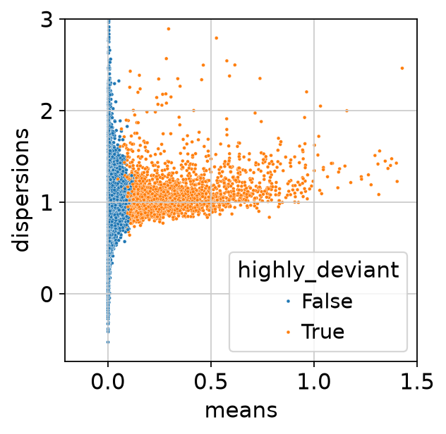
We observe that genes with a high mean expression are selected as highly deviant. This is in agreement with empirical observations by Townes et al., 2019.
af = ln.Artifact.from_anndata(
    adata,
    key="preprocessing_visualization/s4d8_feature_selection.h5ad",
    description="anndata after feature selection",
).save()
af
Output
→ creating new artifact version for key 'preprocessing_visualization/s4d8_feature_selection.h5ad' in storage 's3://lamin-eu-central-1/VPwcjx3CDAa2'
... uploading L5HAg9RzjUS8xFgu0005.h5ad: 0.0%... uploading L5HAg9RzjUS8xFgu0005.h5ad: 1.1%... uploading L5HAg9RzjUS8xFgu0005.h5ad: 2.1%... uploading L5HAg9RzjUS8xFgu0005.h5ad: 3.2%... uploading L5HAg9RzjUS8xFgu0005.h5ad: 4.3%... uploading L5HAg9RzjUS8xFgu0005.h5ad: 8.6%... uploading L5HAg9RzjUS8xFgu0005.h5ad: 11.8%... uploading L5HAg9RzjUS8xFgu0005.h5ad: 20.4%... uploading L5HAg9RzjUS8xFgu0005.h5ad: 21.4%... uploading L5HAg9RzjUS8xFgu0005.h5ad: 22.5%... uploading L5HAg9RzjUS8xFgu0005.h5ad: 29.0%... uploading L5HAg9RzjUS8xFgu0005.h5ad: 33.2%... uploading L5HAg9RzjUS8xFgu0005.h5ad: 39.7%... uploading L5HAg9RzjUS8xFgu0005.h5ad: 44.0%... uploading L5HAg9RzjUS8xFgu0005.h5ad: 51.5%... uploading L5HAg9RzjUS8xFgu0005.h5ad: 54.7%... uploading L5HAg9RzjUS8xFgu0005.h5ad: 60.1%... uploading L5HAg9RzjUS8xFgu0005.h5ad: 62.2%... uploading L5HAg9RzjUS8xFgu0005.h5ad: 65.4%... uploading L5HAg9RzjUS8xFgu0005.h5ad: 71.9%... uploading L5HAg9RzjUS8xFgu0005.h5ad: 76.1%... uploading L5HAg9RzjUS8xFgu0005.h5ad: 81.5%... uploading L5HAg9RzjUS8xFgu0005.h5ad: 83.7%... uploading L5HAg9RzjUS8xFgu0005.h5ad: 86.9%... uploading L5HAg9RzjUS8xFgu0005.h5ad: 93.3%... uploading L5HAg9RzjUS8xFgu0005.h5ad: 96.8%... uploading L5HAg9RzjUS8xFgu0005.h5ad: 100.0%
• replacing the existing cache path /home/lheumos/.cache/lamindb/lamin-eu-central-1/VPwcjx3CDAa2/preprocessing_visualization/s4d8_feature_selection.h5ad
Artifact(uid='L5HAg9RzjUS8xFgu0005', key='preprocessing_visualization/s4d8_feature_selection.h5ad', description='anndata after feature selection', suffix='.h5ad', kind='dataset', otype='AnnData', size=4888582324, hash='wWsHxVmiUwZz1K4T2ePSfn', n_files=None, n_observations=15998, extra_data=None, branch_id=1, created_on_id=1, space_id=1, storage_id=1, run_id=148, schema_id=None, created_by_id=2, created_at=2026-09-29 11:58:22 UTC, is_locked=False, version_tag=None, is_latest=True)Contributors
We gratefully acknowledge the contributions of:
Authors
Anna Schaar
Seo H. Kim
Reviewers
Lukas Heumos
- Townes, F. W., Hicks, S. C., Aryee, M. J., & Irizarry, R. A. (2019). Feature selection and dimension reduction for single-cell term`RNA`-Seq based on a multinomial model. Genome Biology, 20(1), 295. 10.1186/s13059-019-1861-6
- Germain, P.-L., Sonrel, A., & Robinson, M. D. (2020). pipeComp, a general framework for the evaluation of computational pipelines, reveals performant single cell RNA-seq preprocessing tools. Genome Biology, 21(1), 227. 10.1186/s13059-020-02136-7