🧠 Key takeaways
Enrichment analysis needs three inputs (molecular readouts, prior knowledge, and an inference method) and can be run at the single-cell or population level.
Gene sets assume expression reflects protein activity. Footprints use signed, weighted genes reflecting downstream regulatory effects, making them closer to transcriptomics data.
Filter out gene sets with too few members, typically fewer than 10-15 genes, and normalize your data properly before running enrichment.
Competitive tests are generally preferred over self-contained tests, as they rely on a single gene-level statistic and are more stable across samples.
Enrichment results are more sensitive to the choice of gene sets than to the choice of statistical method, so try multiple resources and compare results for concordance.
⚙️ Environment setup
Install conda:
Before creating the environment, ensure that conda is installed on your system.
Save the yml content:
Copy the content from the yml tab into a file named
environment.yml.
Create the environment:
Open a terminal or command prompt.
Run the following command:
conda env create -f environment.yml
Activate the environment:
After the environment is created, activate it using:
conda activate <environment_name>Replace
<environment_name>with the name specified in theenvironment.ymlfile. In the yml file it will look like this:name: <environment_name>
Verify the installation:
Check that the environment was created successfully by running:
conda env list
name: gsea

channels:
  - conda-forge

dependencies:
  - python=3.14.6
  - squidpy=1.8.2
  - scanpy=1.12.3
  - pip
  - pip:
      - "decoupler[full]==2.2.0"
      - lamindb==2.9.1
      - scikit-misc==0.5.2
🗄️ Get data and notebooks
This book uses lamindb to store, share, and load datasets and notebooks using the theislab/sc-best-practices instance. We acknowledge free hosting from Lamin Labs.
Install lamindb
Install the lamindb Python package:
pip install lamindbOptionally create a lamin account
Sign up and log in following the instructions
Verify your setup
Run the
lamin connectcommand:
import lamindb as ln

ln.Artifact.connect("theislab/sc-best-practices").df()
You should now see up to 100 of the stored datasets.
Accessing datasets (Artifacts)
Search for the datasets on the Artifacts page
Load an Artifact and the corresponding object:
import lamindb as ln

af = ln.Artifact.connect("theislab/sc-best-practices").get(
    key="key_of_dataset", is_latest=True
)
obj = af.load()
The object is now accessible in memory and is ready for analysis. Adapt the
lamindb.Artifact.connect("theislab/sc-best-practices").get("SOMEIDXXXX")suffix to get respective versions.Accessing notebooks (Transforms)
Search for the notebook on the Transforms page
Load the notebook:
lamin load <notebook url>which will download the notebook to the current working directory. Analogously to
Artifacts, you can adapt the suffix ID to get older versions.
Motivation
Single-cell RNA-seq (scRNA-seq) provides unprecedented insights into molecular variation, but it is hard to interpret the resulting high-dimensional data, since hundreds of genes may explain the observed variability in a particular biological context.
Gene set enrichment analysis (GSEA) allows to summarize the high-dimensional molecular measurements into interpretable terms such as biological processes or pathways, which enable a better understanding of the obtained results and the generation of mechanistic hypothesis. Note that GSEA is also known as pathway analysis, enrichment analysis, gene set analysis and functional analysis. Accordingly, we use these terms interchangeably throughout this chapter.
Functional analysis requires three different inputs:
Molecular readouts: a matrix containing gene expression or gene-level statistics (log fold changes, test statistic).
Prior knowledge: collection of gene sets or footprints associated to biological processes (e.g. epithelial to mesechymal transition, metabolism etc.) or regulatory pathways (e.g. MAPK signalling).
Inference method: statistical method that computes the “enrichment” scores of the gene sets from the molecular data.
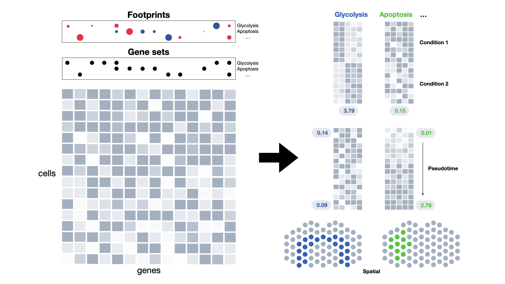
Figure 1:Gene set enrichment analysis can generate enrichment scores across conditions, time, and space. Numbers represent enrichment scores for glycolysis (blue) and apoptosis (green).
Background
Gene set collections
Gene sets are a curated list of genes that are known to be involved in a biological process through previous studies and/or experiments and are stored in prior knowledge databases. The Molecular Signatures Database (MSigDB) Subramanian et al., 2005Liberzon et al., 2011 is the most comprehensive database consisting of 9 collections of gene sets. Some commonly used collections are C5, which is the gene ontology (GO) collection, C2 collection of curated gene signatures from published studies that are typically context (e.g. tissue, condition) specific, but also include KEGG and REACTOME gene signatures. The Hallmark collection were developed to reduce the redundancy between gene sets, and for immunologic studies the C7 collection is a common choice. Note that these signatures are mainly derived from Bulk-seq measurements and measure continuous phenotypes. Recently and with the wide-spread availability of scRNA-seq datasets, databases have evolved that provide curated marker lists derived from published single cell studies that define cell types in various tissues and species. These include CellMarker Zhang et al., 2019 and PanglaoDB Franzén et al., 2019. Curated marker lists are not limited to those made available in databases, and can be curated by oneself using own or public data.
Gene sets contain experimentally validated protein members of a given pathway. Running enrichment on those assumes a strong correlation between gene expression, protein abundance, and protein activity. Despite this, most gene sets still provide reliable scores because their members are usually regulated together Szalai & Saez-Rodriguez, 2020. On the other hand, footprints are sets that instead contain genes that changed downstream of said process when it was active, bringing them closer to transcriptomics data. Footprints usually contain interaction weights for each gene in the set, denoting its strength and mode of regulation (positive: activation, negative: inhibition). This concept has been applied to transcription factors, kinases and enzymes Dugourd & Saez-Rodriguez, 2019. Known databases of footprints include PROGENy Schubert et al., 2018 for signaling pathways, CytoSig Jiang et al., 2021 for ligand signatures, and DoRothEA Garcia-Alonso et al., 2019 for transcription factors. Similar to gene sets, these can be curated by oneself derived in a data-driven manner, for example by generating Gene Regulatory Networks.
Applications in single-cell data
In scRNA-seq data analysis, enrichment is generally carried out on clusters of cells or cell types, one-at-a-time. For example, one can test how genes change between untreated and treated cells per cell-type and use the obtained gene statistics to see what biological processes are deregulated Squair et al., 2021Crowell et al., 2020. Enrichment can be assessed in any complex experimental design while accounting for batch effects, between-individual variations, gender, strain differences in mouse models, etc. (check the differential gene expression analysis chapter for best practices).
Alternatively, enrichment methods can also be applied directly to the gene expression data of individual cells with the main objective to reduce highly-dimensional expression data into a collection of interpretable latent variables to explore their variability. This dimensionality reduction driven by prior knowledge captures transcriptional heterogeneity and variability at the single-cell level, increasing the power of population comparisons, while keeping biological significance. Compared to other data-driven dimensionality reduction methods like principal component analysis (PCA) or factor analysis, the estimated latent variables generated from enrichment methods are not necessarily independent.
Most enrichment methods have been previously developed for bulk RNA-seq but can be applied to single-cell data. Holland et al. (2020) found that methods have optimal performance in simulated scRNA-seq data, and even partially outperform tools specifically designed for scRNA-seq analysis despite the drop-out events and low library sizes in single-cell data. Holland et al. also concluded that enrichment inference is more sensitive to the choice of gene sets (the prior knowledge used) rather than the statistical methods. This observation though can be explained by the fact that biological processes might be context-specific; for example TF-target associations in one cell-type may actually differ from another cell-type or tissue. There are different strategies to contextualize gene sets, such as inferring gene regulatory networks, or performing factor analysis influenced by prior, as seen in Muvi Qoku & Buettner, 2022 and Spectra Kunes et al., 2022.
In contrast to Holland et al., Zhang et al. Zhang et al. (2020) found that single-cell-based tools, specifically Pagoda2, outperform some bulk-base methods from three different aspects of accuracy, stability and scalability. It should be noted that functional inference tools inherently do not account for batch effects or biological variations other than the biological variation of interest. Therefore, it is up to the data analyst to ensure that the differential gene expression analysis step has worked properly.
Enrichment methods
Most enrichment methods are based on hypergeometric tests, rank statistics or empirical estimations of likelihoods based on permutations. Regardless of the statistical method used, their hypothesis tests can be divided in two main classes: competitive or self-contained as defined by Goeman & Bühlmann (2007). A competitive test tests whether the genes in the set are highly ranked relative to the genes not in the set (usually of the same size). The sampling unit here is genes, so the test can be done with a single sample or contrast vector. In self-contained gene set testing, the sampling unit is the subject, so multiple samples per group are required, but it is not required to have genes that are not present in the set. A self-contained test tests whether genes in the test set are differentially expressed without regard to any other gene measured in the dataset. Competitive hypotheses are the most used in enrichment analysis because they depend solely on a single vector of gene-level statistics compared to self-contained methods which are limited by the number of samples Mathur et al., 2018. In a recent benchmark Geistlinger et al., 2020, it has been shown that self-contained methods might be quite sensitive since they can identify gene sets as enriched while containing only a single differentially expressed gene. On the other hand, competitive methods might be more restrictive by testing for excess of differential expression in the gene set when compared to the background level, coming closer to the intuition of an enrichment and tend to rank relevant gene sets systematically higher than self-contained methods. However, it is important to keep in mind that each approach has its pros an cons and that these distinctions between the two null hypotheses mainly affect the interpretation of gene set enrichment results. In practice, competitive methods dominate for their stability, since removing even a single sample can swing self-contained results. For this reason, we will only work with competitive methods in this chapter.
Common competitive enrichment methods include simple hypergeomtric tests or one-tailed Fisher’s exact test (as in Enrichr Chen et al., 2013), the GSEA algorithm Subramanian et al., 2005 and its fast implementation (fgsea) Korotkevich et al., 2021, GSVA Hänzelmann et al., 2013, VISION DeTomaso et al., 2019, AUCell Aibar et al., 2017, Pagoda2 Fan et al., 2016Lake et al., 2018, camera (as in limma Ritchie et al., 2015), scDECAF and simple combined z-score Lee et al., 2008. As mentioned before, while less computational tools that implement these methods use self-contained hypothesis tests, notable examples are roast and fry, both available in the differential testing framework limma Ritchie et al., 2015. These methods leverage linear models and Empirical Bayes moderation of test statistics Smyth, 2005. Note that while most methods work downstream of differential gene testing, methods included in the limma framework (camera, roast and fry) start from the sample level gene expression data. Detailed explanations on these methods can be found in the limma user manual.
There are also enrichment methods that leverage footprints when inferring scores, i.e. they accommodate the usage of gene weights. Common competitive enrichment methods that leverage footprints include VIPER Alvarez et al., 2016, ULM and MLM Badia-i-Mompel et al., 2022. For self-contained enrichment methods, fry and roast do it too.
Enrichment frameworks collect several enrichment methods in a single tool. These facilitate the usage of various enrichment methods on the data since they have a common format and provide utility functions to access prior knowledge resources. Some of them are Piano Väremo et al., 2013 and EGSEA Alhamdoosh et al., 2016 (available in R), and decoupler Badia-i-Mompel et al., 2022 (available both in R and Python).
| Method | Type of Null Hypothesis | Weights genes | Reference |
|---|---|---|---|
| Fisher’s exact test | Competitive | No | Chen et al., 2013 |
| GSEA | Competitive | No | Subramanian et al., 2005Korotkevich et al., 2021 |
| GSVA | Competitive | No | Hänzelmann et al., 2013 |
| VISION | Competitive | No | DeTomaso et al., 2019 |
| AUCell | Competitive | No | Aibar et al., 2017 |
| Pagoda2 | Competitive | No | Fan et al., 2016Lake et al., 2018 |
| Camera | Competitive | No | Ritchie et al., 2015 |
| Z-score | Competitive | No | Lee et al., 2008 |
| Roast | Self-constrained | Yes | Ritchie et al., 2015 |
| Fry | Self-constrained | Yes | Ritchie et al., 2015 |
| VIPER | Competitive | Yes | Alvarez et al., 2016 |
| ULM | Competitive | Yes | Badia-i-Mompel et al., 2022 |
| MLM | Competitive | Yes | Badia-i-Mompel et al., 2022 |
Technical considerations
Filtering out the gene sets with low number of genes
A common practice is to exclude any gene sets with a few genes overlapping the data or Highly Variable Genes (HVG) in the pre-processing step. Zhang et al. (2020) found that the performance of both single-cell-based and bulk-based methods drops as gene coverage, that is the number of genes in pathways/gene sets, decreases. Holland et al. (2020) also found that gene sets of smaller size adversely impacts the performance of Bulk-seq enrichment methods on single cell data. These report collectively support that filtering gene sets with few gene members, say less than 10 or 15 genes in the set, is beneficial in functional analysis. Damian & Gorfine (2004) attributed this to the fact that gene variances in gene sets with a smaller number of genes are more likely to be large, whereas gene variances in larger gene sets tend to be smaller. This impacts the accuracy of the test statistics computed to test for enrichment. Zhang et al. additionally found that pathway analysis was susceptible to normalization procedures applied to gene expression measurements.
Data normalization
Read counts in single cell experiments are typically normalised early on in the pre-processing pipeline to ensure that measuerments are comparable across cells of various library sizes. Zhang et al. (2020) found that normalisation by SCTransform Hafemeister & Satija, 2019 and scran Lun et al., 2016 generally improves the performance of both single-cell- and bulk-based enrichment scoring tools. They found that the performance of AUCell (a rank-base method) and z-score (transformation to zero mean, unit standard deviation) is particularly affected by normalization with distinct methods.
Functional analysis between conditions
Prepare and explore the data
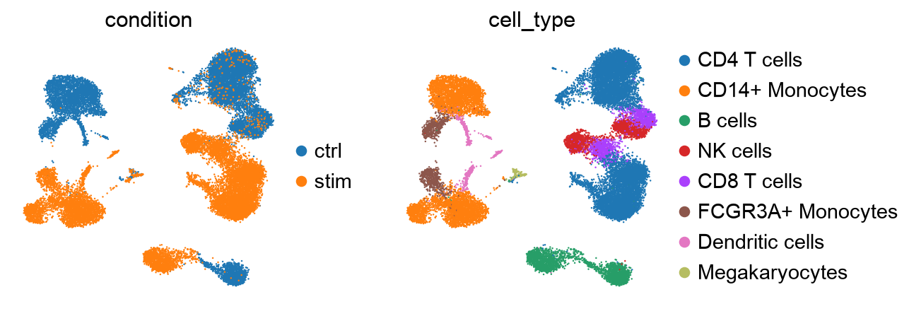
We first download the 25K PBMC data and follow the standard scanpy workflow for normalization of read counts and subsetting on the highly variable genes. The dataset contains untreated and IFN- stimulated human PBMC cells Kang et al., 2018. We explore patterns of variation in the data with UMAP representation of 4000 highly variable genes.
import decoupler as dc
import lamindb as ln
import matplotlib.pyplot as plt
import scanpy as sc
import squidpy as sq

sc.set_figure_params(figsize=(3, 3), frameon=False)

ln.connect("theislab/sc-best-practices")

ln.track("zTql6b4pzLB3")
Output
→ loaded Transform('zTql6b4pzLB30002', key='gsea_pathway.ipynb'), re-started Run('BBv1A3z2d7rChepQ') at 2026-08-14 12:13:30 UTC
→ notebook imports: decoupler==2.2.0 lamindb-core==2.9.1 matplotlib==3.11.1 scanpy==1.12.3 squidpy==1.8.2
• tip: to identify the notebook across renames, pass the uid: ln.track("zTql6b4pzLB3")
adata = ln.Artifact.get(
    key="conditions/differential_gene_expression.h5ad",
).load()
adata
AnnData object with n_obs × n_vars = 24673 × 15706
obs: 'nCount_RNA', 'nFeature_RNA', 'tsne1', 'tsne2', 'label', 'cluster', 'cell_type', 'replicate', 'nCount_SCT', 'nFeature_SCT', 'integrated_snn_res.0.4', 'seurat_clusters'
var: 'name'
obsm: 'X_pca', 'X_umap'
layers: None (.X)# Storing the counts for later use
adata.layers["counts"] = adata.X.copy()
# Renaming label to condition
adata.obs = adata.obs.rename({"label": "condition"}, axis=1)
# Normalizing
sc.pp.normalize_total(adata)
sc.pp.log1p(adata)# Finding highly variable genes using count data
sc.pp.highly_variable_genes(
adata, n_top_genes=4000, flavor="seurat_v3", subset=False, layer="counts"
)While the current object comes with UMAP and PCA embeddings, these have been corrected for stimulation condition, which we don’t want for this analysis. Instead we will recompute these.
sc.pp.pca(adata)
sc.pp.neighbors(adata)
sc.tl.umap(adata)
sc.pl.umap(
adata,
color=["condition", "cell_type"],
frameon=False,
ncols=2,
)
Retrieving gene sets
Gene sets can be downloaded from their respective databases, usually they are stored in the GMT file format.
Gene sets can also be retrieved from databases using wrappers, here is an example on how to download MSigDB using decoupler (which leverages the meta-database OmniPath Türei et al., 2021):
# Retrieving via python
msigdb = dc.op.resource("MSigDB", organism='human')

# Get reactome pathways
reactome = msigdb.query("collection == 'reactome_pathways'")
# Filter duplicates
reactome = reactome[~reactome.duplicated(("geneset", "genesymbol"))]
However, for stability of this tutorial we are using a fixed version of the gene set collection. Here we download and read the GMT file for the REACTOME pathways annotated in the C2 collection of MSigDB:
gmt = ln.Artifact.get(
    key="conditions/gsea_pathway/c2.cp.reactome.v7.5.1.symbols.gmt",
).cache()

reactome = dc.pp.read_gmt(gmt)
reactomeHere we remove potential noisy gene sets by removing sets with too low (<15) or too high (>500) number of members. Note that these values are completely arbitrary and should be adjusted to the question at hand. As a rule of thumb, we recommend exploring the distribution of gene set lengths to get an idea if there are any outliers.
geneset_size = reactome.groupby("source").size()
reactome = reactome.loc[
    [15 < geneset_size.loc[gset] < 500 for gset in reactome["source"]]
]
reactomeCell-level gene set scoring
As previously described, gene set scores can be inferred in each individual cell, that is based on absolute gene expression in the cell, regardless of expression of genes in the other cells.
Inference using gene sets with AUCell
To demonstrate this concept, we will start by using the method AUCell Aibar et al., 2017 through decoupler.
dc.mt.aucell(
    data=adata,
    net=reactome,
    raw=False,
)

adata
AnnData object with n_obs × n_vars = 24673 × 15706
obs: 'nCount_RNA', 'nFeature_RNA', 'tsne1', 'tsne2', 'condition', 'cluster', 'cell_type', 'replicate', 'nCount_SCT', 'nFeature_SCT', 'integrated_snn_res.0.4', 'seurat_clusters'
var: 'name', 'highly_variable', 'highly_variable_rank', 'means', 'variances', 'variances_norm'
uns: 'log1p', 'hvg', 'pca', 'neighbors', 'umap', 'condition_colors', 'cell_type_colors'
obsm: 'X_pca', 'X_umap', 'score_aucell'
varm: 'PCs'
obsp: 'distances', 'connectivities'
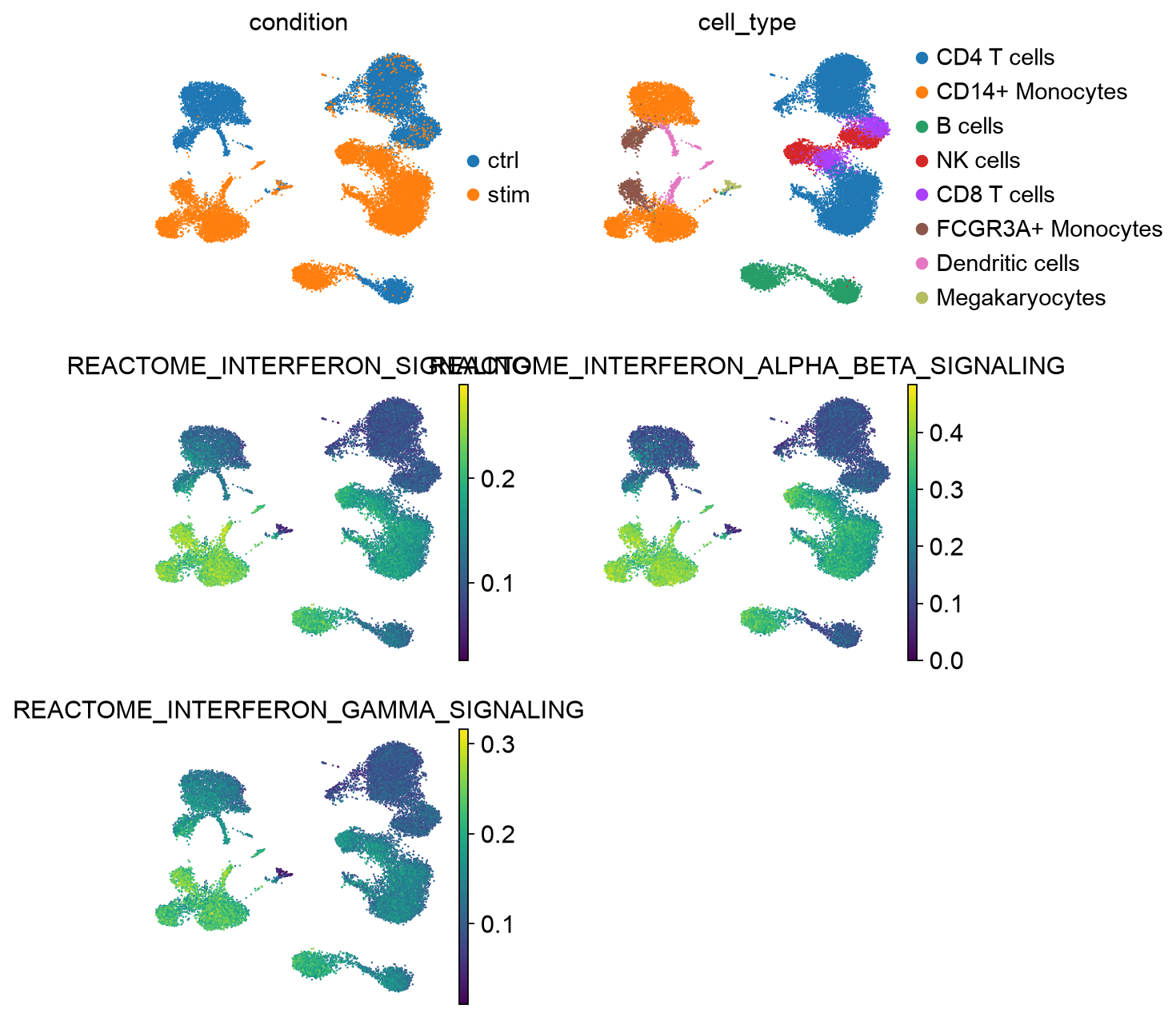
layers: None (.X), 'counts'We now add the scores for the interferon-related REACTOME pathways to the obs field of the AnnData object and annotate the score level of these pathways in each of the cells on the UMAP:
ifn_pathways = [
    "REACTOME_INTERFERON_SIGNALING",
    "REACTOME_INTERFERON_ALPHA_BETA_SIGNALING",
    "REACTOME_INTERFERON_GAMMA_SIGNALING",
]

adata.obs[ifn_pathways] = adata.obsm["score_aucell"][ifn_pathways]
sc.pl.umap(
adata,
color=["condition", "cell_type"] + ifn_pathways,
frameon=False,
ncols=2,
wspace=0.3,
)
We can also visualize this as distributions in violinplots:
sc.pl.stacked_violin(
    adata,
    var_names=ifn_pathways,
    groupby=["cell_type", "condition"],
    swap_axes=True,
    figsize=(12, 3),
)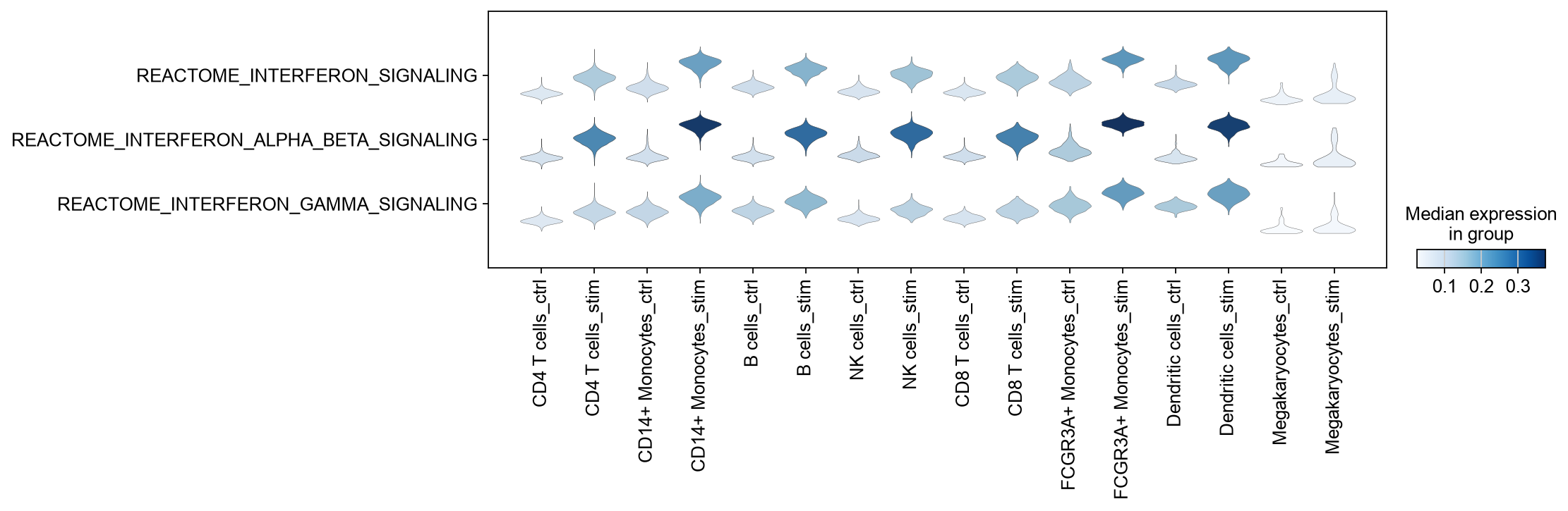
AUCell scores the pathways well-known to be implicated in interferon signalling high in IFN-stimulated cells (except for Megakaryocytes which is expected), while cells in the control condition generally have lower scores for these pathways, demonstrating that gene set scoring with AUCell has been successful.
Inference using footprints with ULM
Additionally, we can infer scores using footprints instead of gene sets.
Here we will leverage the database PROGENy Schubert et al., 2018.
Here is how to access it through decoupler:
# Retrieving via python
progeny = dc.op.progeny(organism='human', top=100)
However, again for stability of this tutorial we are using a fixed version.
progeny = ln.Artifact.get(key="conditions/gsea_pathway/progeny.parquet").load()
progenyNote that in this resource, each gene has a weight associated to the pathway it belongs, denoting its mode of regulation (positive or negative) and its importance.
Now lets estimate pathway scores using ULM from decoupler, a method that accounts for weighted gene sets:
dc.mt.ulm(
    data=adata,
    net=progeny,
    raw=False,
)
adata
AnnData object with n_obs × n_vars = 24673 × 15706
obs: 'nCount_RNA', 'nFeature_RNA', 'tsne1', 'tsne2', 'condition', 'cluster', 'cell_type', 'replicate', 'nCount_SCT', 'nFeature_SCT', 'integrated_snn_res.0.4', 'seurat_clusters', 'REACTOME_INTERFERON_SIGNALING', 'REACTOME_INTERFERON_ALPHA_BETA_SIGNALING', 'REACTOME_INTERFERON_GAMMA_SIGNALING'
var: 'name', 'highly_variable', 'highly_variable_rank', 'means', 'variances', 'variances_norm'
uns: 'log1p', 'hvg', 'pca', 'neighbors', 'umap', 'condition_colors', 'cell_type_colors'
obsm: 'X_pca', 'X_umap', 'score_aucell', 'score_ulm', 'padj_ulm'
varm: 'PCs'
obsp: 'distances', 'connectivities'
layers: None (.X), 'counts'Next we add the scores for the immune-related PROGENy pathways to the obs field of the AnnData object and annotate the score level of these pathways in each of the cells on the UMAP:
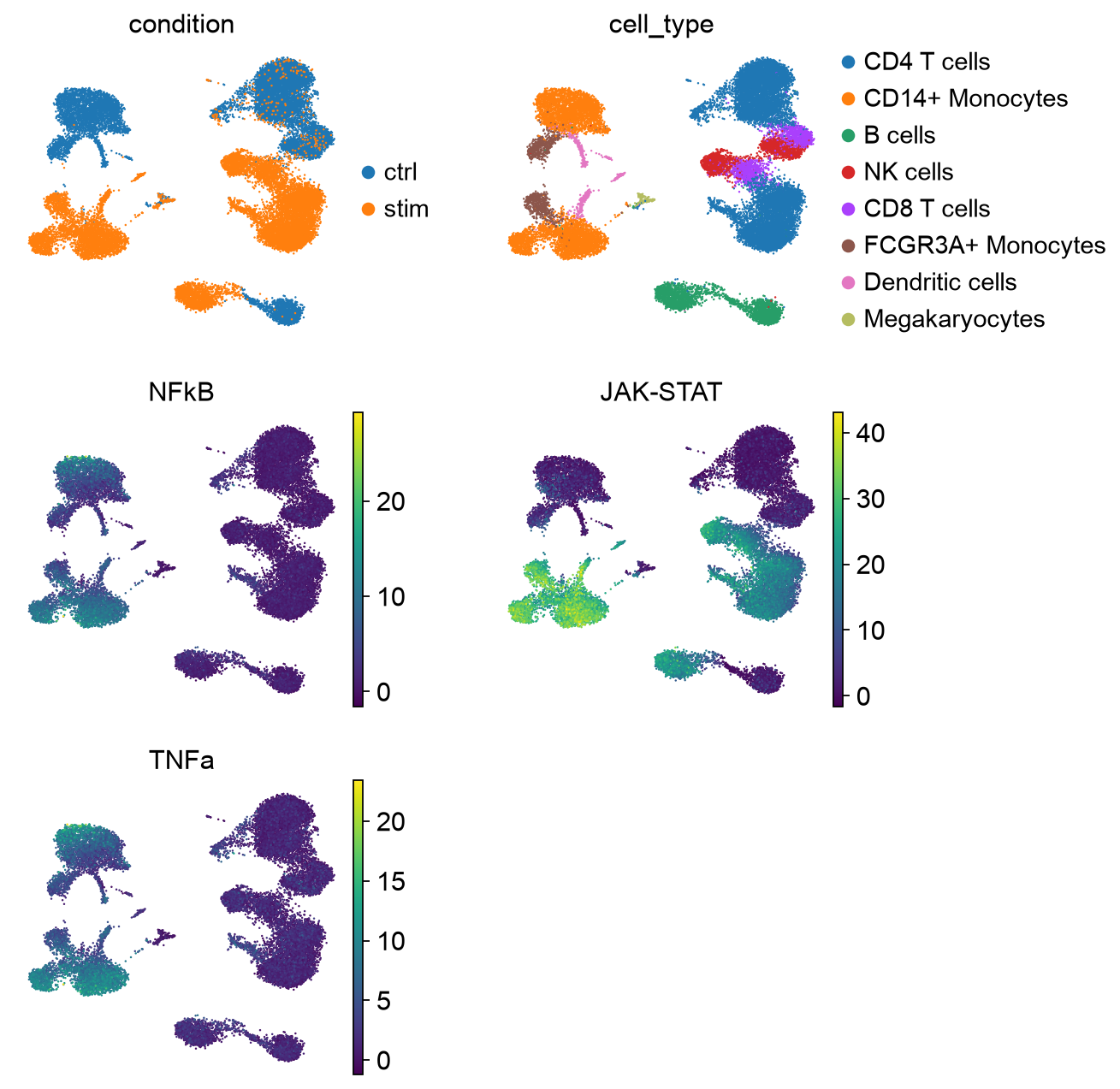
imun_pathways = ["NFkB", "JAK-STAT", "TNFa"]

adata.obs[imun_pathways] = adata.obsm["score_ulm"][imun_pathways]
sc.pl.umap(
adata,
color=["condition", "cell_type"] + imun_pathways,
frameon=False,
ncols=2,
wspace=0.3,
)
As before, we can also visualize this in violinplots:
sc.pl.stacked_violin(
    adata,
    var_names=imun_pathways,
    groupby=["cell_type", "condition"],
    swap_axes=True,
    figsize=(12, 3),
)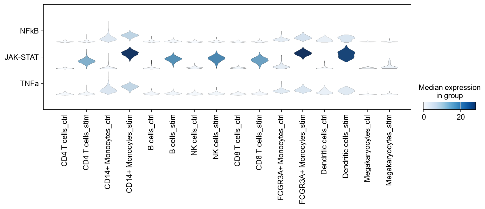
In this case, the pathway JAK-STAT, triggered by the binding of interferons such as INF-, is the one with the highest score after stimulation. The other immune pathways, NFkB and TNFa, remain overall the same. The concordance between pathway scores by AUCell and ULM is promising, given that we know a priori that IFN-related pathways should be the top-ranked terms.
Population contrast enrichment scoring
Previously, we enriched functional terms for individual cells.
Now, we instead compare cell populations.
For this, we pseudobulk our samples and cell type combinations and perform DGE on these pseudobulks to mitigate inflated p-values Squair et al., 2021.
We use pydeseq2 for the DGE analysis.
Since this analysis builds on a standard DGE workflow, see the DGE analysis chapter if you haven’t run DGE on your data yet. In this tutorial, we load the previously computed DGE results for CD14+ monocytes across conditions.
res_df = ln.Artifact.get(
    key="conditions/differential_gene_expression/res_df_CD14_Monocytes.parquet"
).load()
res_dfWhile any statistic can be used, we recommend using t-values rather than log2FCs, as t-values account for the significance of the change.
We will transform the obtained t-values, stored in the column "stat", into a wide matrix format so that it can be used with decoupler.
res_df = res_df.set_index("variable")
data = res_df[["stat"]].T.rename(index={"stat": "stim.vs.ctrl"})
dataInference using gene sets with GSEA
Once we prepared our gene statistics, we will use those to infer pathway scores using GSEA Subramanian et al., 2005 from decoupler.
Running dc.mt.gsea will return enrichment scores and adjusted p-values using Benjamini-Hochberg.
score, padj = dc.mt.gsea(data=data, net=reactome)

mask = (padj.T < 0.05).iloc[:, 0]
score = score.loc[:, mask]
scoreWe can then visualize the most active and inactive pathways.
fig = dc.pl.barplot(data=score, name="stim.vs.ctrl", top=15, return_fig=True)

ax = fig.axes[0]
ax.tick_params(axis="y", labelsize=8)
plt.show()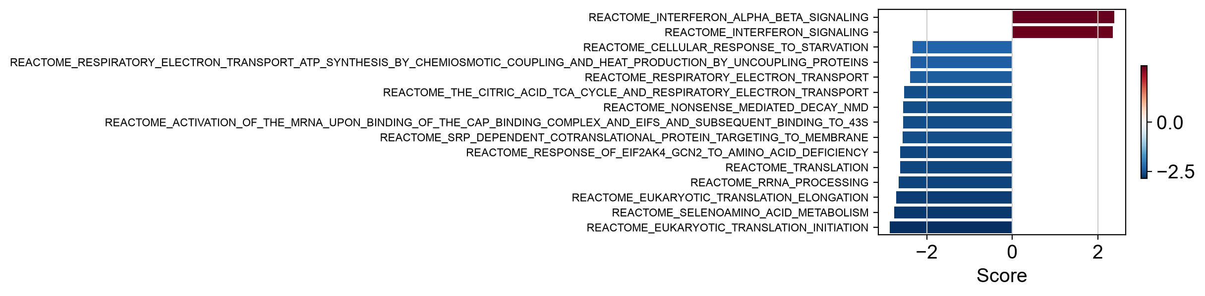
Pathways are shown on the y-axis, and the x-axis shows the GSEA enrichment score. Enrichment scores are signed: positive scores indicate pathway upregulation, while negative scores indicate downregulation. Larger absolute values indicate stronger enrichment. Only the top 15 pathways are displayed, ranked by direction and magnitude. The majority of interferon-related pathways are indeed positively ranked and in the right direction.
Inference using footprints with ULM
Let us leverage DGE result again, but this time with the PROGENy footprints and the ULM method.
score, padj = dc.mt.ulm(data=data, net=progeny)
mask = (padj.T < 0.05).iloc[:, 0]
score.loc[:, mask]Like in GSEA, using ULM returns enrichment scores and adjusted p-values using Benjamini-Hochberg. Scores are signed and show the magnitute of up- or downregulation. While only JAK-STAT and NFkB show significant results, we want to plot all 13 pathways available in PROGENy:
dc.pl.barplot(
    data=score,
    name="stim.vs.ctrl",
)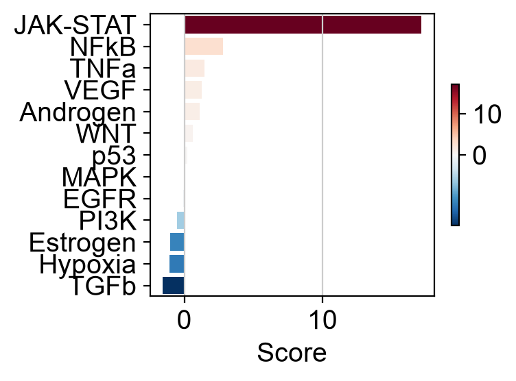
As seen in the previous section, JAK-STAT, a INF- induced pathway, is the one with the highest score in stimulated CD14+ monocytes compared to the control ones.
Pseudotime Enrichment Scoring
Analyzing omics data is not always limited to comparing two discrete groups, such as treatment versus control. Many biological processes, including cell differentiation, disease progression, and development, are continuous. In these cases, it is important to evaluate how features and their enrichment scores change along the continuous trajectory.
We apply this approach to the adult human bone marrow dataset Setty et al., 2019 from a previous chapter, where we concluded that the Palantir pseudotime should be used for subsequent analyses.
adata = ln.Artifact.get(key="trajectories/pseudotemporal/bonemarrow_result.h5ad").load()
adata
AnnData object with n_obs × n_vars = 5780 × 11975
obs: 'clusters', 'palantir_pseudotime', 'palantir_diff_potential', 'dpt_pseudotime'
var: 'palantir', 'n_counts', 'highly_variable', 'means', 'dispersions', 'dispersions_norm'
uns: 'clusters_colors', 'diffmap_evals', 'hvg', 'iroot', 'log1p', 'neighbors', 'palantir_branch_probs_cell_types', 'pca'
obsm: 'MAGIC_imputed_data', 'X_diffmap', 'X_pca', 'X_tsne', 'palantir_branch_probs'
varm: 'PCs'
obsp: 'connectivities', 'distances'
layers: 'spliced', 'unspliced', None (.X)Here, instead of using gene sets representing specific pathways, we score transcription factors (TFs) based on gene regulatory networks (GRNs). TFs are genes whose protein products bind DNA and regulate the expression of target genes, either promoting or inhibiting transcription. Because TF transcript levels often do not reflect their actual activity, we assess TF activity through enrichment of their target genes Badia-i-Mompel et al., 2023. GRNs capture these TF-gene interactions and therefore provide a more accurate representation of regulatory activity. Again, the scores are signed and reflect the magnitude of the effect, indicating the extent to which TFs are activated or deactivated. For more details, please see our GRN chapter.
To do so, we use the CollecTRI network, a comprehensive resource containing a curated collection of TFs and their target genes Müller-Dott et al., 2023.
The network can be accessed through decoupler as follows:
collectri = dc.op.collectri(organism="human")As before, to ensure the stability and reproducibility of this tutorial, we use a fixed version of the network.
collectri = ln.Artifact.get(key="conditions/gsea_pathway/collectri.parquet").load()
collectriTF scores can be easily computed by running the ulm method.
dc.mt.ulm(data=adata, net=collectri)Scores can then be extracted as a new AnnData object.
score = dc.pp.get_obsm(adata=adata, key="score_ulm")
score
AnnData object with n_obs × n_vars = 5780 × 598
obs: 'clusters', 'palantir_pseudotime', 'palantir_diff_potential', 'dpt_pseudotime'
uns: 'clusters_colors', 'diffmap_evals', 'hvg', 'iroot', 'log1p', 'neighbors', 'palantir_branch_probs_cell_types', 'pca'
obsm: 'MAGIC_imputed_data', 'X_diffmap', 'X_pca', 'X_tsne', 'palantir_branch_probs', 'score_ulm', 'padj_ulm'
layers: None (.X)Next, TFs associated with the inferred pseudotime can be identified.
tfs = dc.tl.rankby_order(
    adata=score,
    order="palantir_pseudotime",
    stat="dcor",
)
tfsThe top 5 TF markers associated to the pseudotime can then be extracted.
top_tfs = tfs.head(5)["name"].to_list()
top_tfs
['TFDP1', 'POU3F2', 'NKX2-2', 'LEF1', 'FOSB']And visualized.
score.obs["clusters"].unique()['Ery_1', 'HSC_1', 'Mono_1', 'Precursors', 'Mega', 'HSC_2', 'Mono_2', 'Ery_2', 'DCs', 'CLP']
Categories (10, object): ['HSC_1', 'HSC_2', 'Ery_1', 'Mono_1', ..., 'Mono_2', 'DCs', 'Ery_2', 'Mega']sc.pl.tsne(
score,
color=top_tfs + ["clusters", "palantir_pseudotime"],
ncols=2,
color_map="gnuplot2",
)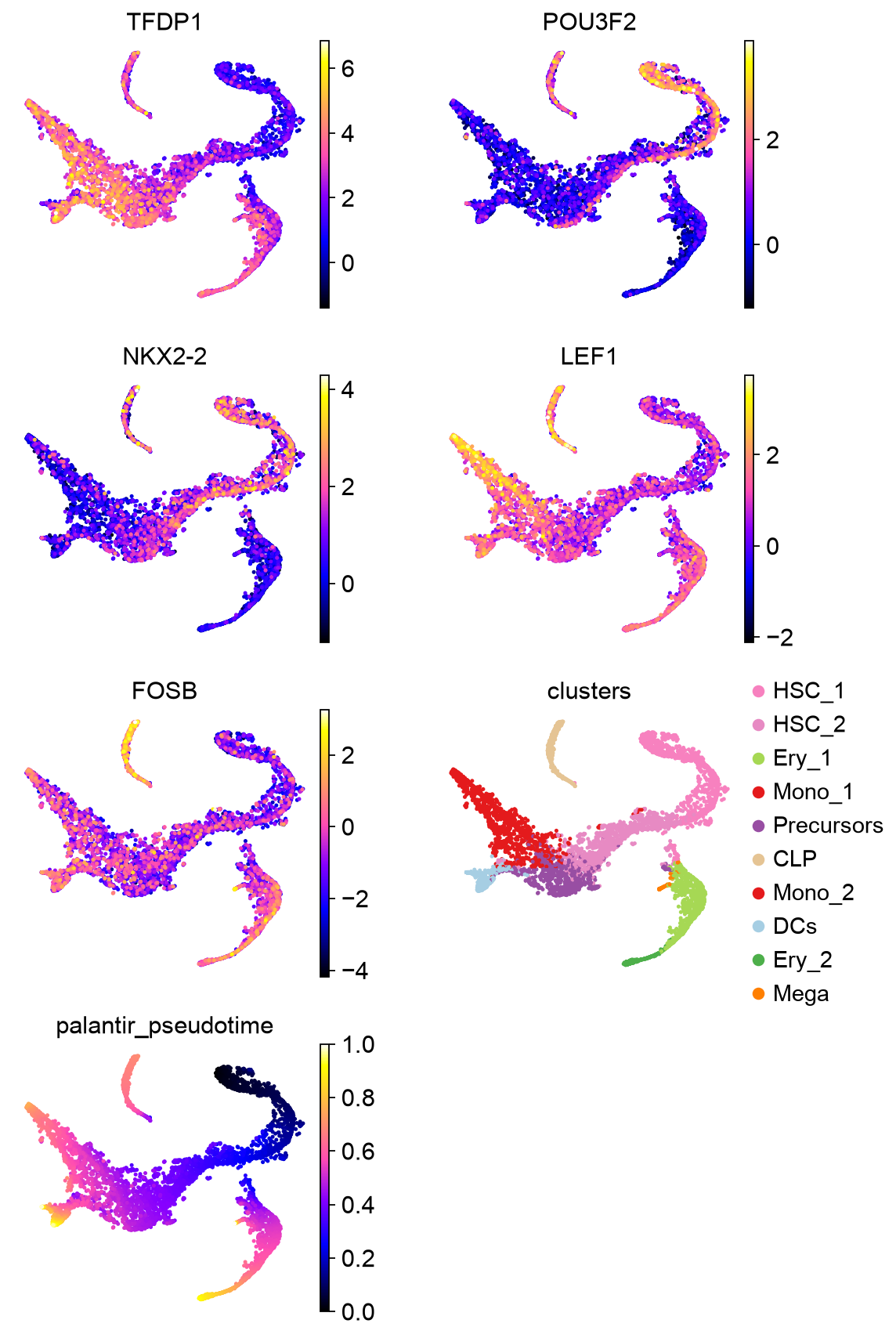
For example, LEF-1 plays a pivotal role in lymphoid differentiation Petropoulos et al., 2008, making its activation in common lymphoid progenitors (CLPs) biologically plausible. Among other factors, FOSB, a subunit of AP-1, plays a role in the functional development of hematopoietic precursor cells into mature blood cells, supporting increased activation at later pseudotime points Liebermann et al., 1998.
Prior to generating more complex visualizations, cells are grouped into bins based on their ordering to facilitate plotting.
bin_tfs = dc.pp.bin_order(
    adata=score,
    order="palantir_pseudotime",
    names=top_tfs,
    label="clusters",
)
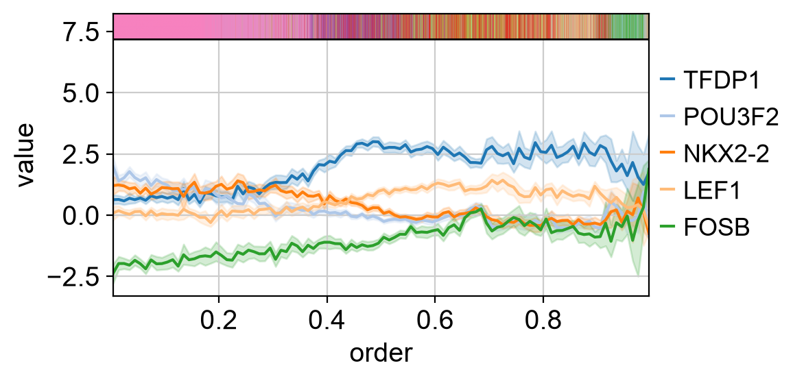
bin_tfsWhich can be plotted as lines.
dc.pl.order(
    df=bin_tfs,
    mode="line",
    figsize=(6, 3),
)
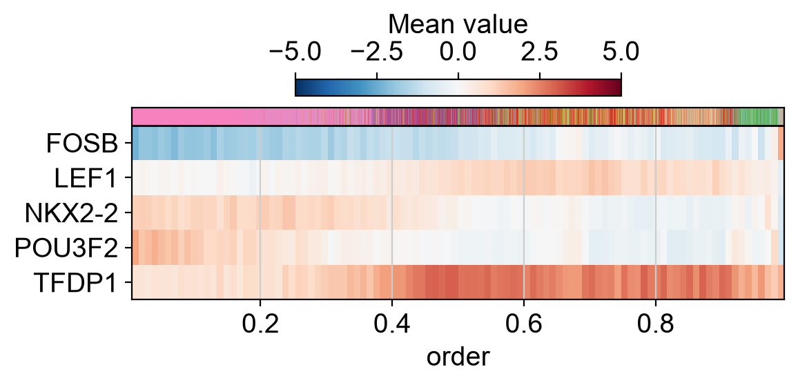
Or as a matrix.
dc.pl.order(
    df=bin_tfs,
    mode="mat",
    kw_order={"vmin": -5, "vmax": +5, "cmap": "RdBu_r"},
    figsize=(6, 3),
)
Additionally, to better understand the obtained enrichment scores, the targets of a specified TF can be plotted along the trajectory.
dc.pl.order_targets(
    adata=adata,
    net=collectri,
    label="clusters",
    source="FOSB",
    order="palantir_pseudotime",
)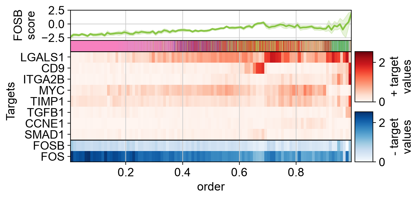
The change in the enrichment score results from positive targets of FOSB increasing in expression, while its repressed targets decrease in expression along the trajectory. Consequently, the TF is inactive at the beginning but becomes active by the end.
Spatial Enrichment Analysis
Finally, we can also perform GSEA on spatial transcriptomics data. The dataset we use comprises approximately 4,000 mini-bulks (spots) for ~15k genes from a chronic active multiple sclerosis lesion, profiled using Visium Lerma-Martin et al., 2024. Here, we again aim to characterize TF activity using CollecTRI, but this time in its spatial context.
adata = ln.Artifact.get(key="conditions/gsea_pathway/msvisium.h5ad").load()
adata
AnnData object with n_obs × n_vars = 3839 × 14940
obs: 'array_row', 'array_col', 'niches'
uns: 'spatial'
obsm: 'spatial'
layers: None (.X)The following step normalizes the data and stores it into a layer for later use.
sc.pp.normalize_total(adata, target_sum=1e4)
sc.pp.log1p(adata)

adata.layers["norm"] = adata.X.copy()
The spot metadata stored in obs can be inspected.
adata.obsThe dataset also includes tissue annotations from the original publication:
GM: Grey Matter
LC: Lesion Core
LR: Lesion Rim
PPWM: PeriPlaque White Matter
VI: Vascular Infiltrating
The H&E image and the different annotated regions (niches) can be visualized.
adataAnnData object with n_obs × n_vars = 3839 × 14940
obs: 'array_row', 'array_col', 'niches'
uns: 'spatial', 'log1p'
obsm: 'spatial'
layers: None (.X), 'norm'sq.pl.spatial_scatter(adata, color=[None, "niches"], size=1.5, ncols=1)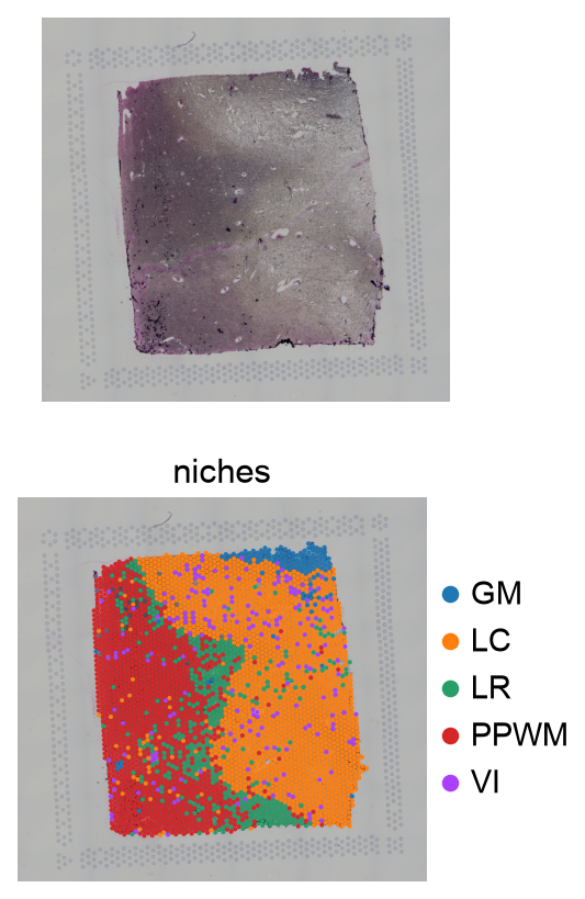
Spatial Weighting
Spatial data are often sparse. To address this, spatial information can be leveraged to impute gene expression based on the expression levels of nearby spatial neighbors Dimitrov et al., 2024. This is achieved by generating spatial weights for each spot and applying them to the gene expression values, effectively smoothing the data.
dc.pp.knn(adata, key="spatial", bw=100, cutoff=0.1)The spatial weights assigned to each spot can then be visualized.
# Plot the spatial weights of one spot
adata.obs["conn"] = adata.obsp["spatial_connectivities"][0].toarray().ravel()
sq.pl.spatial_scatter(adata, color="conn", size=1.5)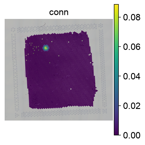
It can be observed that for a given spot, the spatial weight is maximal at the spot itself and decreases with increasing distance to other spots.
Adjust the bandwith (bw) to increase or decrease the radius to consider.
The gene expression values can now be spatially weighted.
# Update X with spatially weighted gene exression
adata.X = adata.obsp["spatial_connectivities"].dot(adata.X)
The original log-normalized counts can be plotted alongside the newly spatially transformed values.
genes = ["MOG", "CD163", "IGKC"]

# Log-normalized counts
sq.pl.spatial_scatter(adata, color=genes, size=1.5, layer="norm")

# Spatially weighted gene expression
sq.pl.spatial_scatter(adata, color=genes, size=1.5)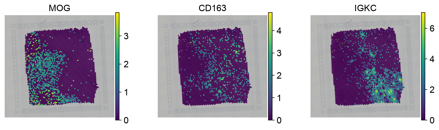
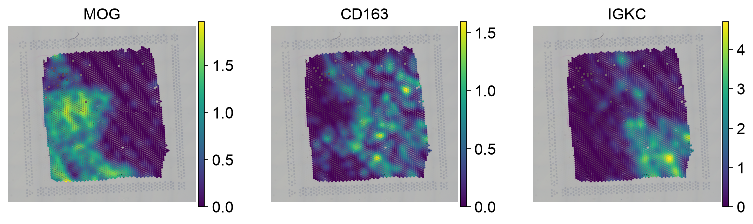
After smoothing, spots surrounded by other spots expressing the same gene will have higher values compared to spots lacking neighboring spots with high values, even if those spots themselves had high values of expression.
Gene expression for these genes appears to exhibit spatial compartmentalization.
Scoring
We can now again use the ulm method to compute TF scores using collectri, which we loaded previously.
dc.mt.ulm(data=adata, net=collectri)And extract the scores.
score = dc.pp.get_obsm(adata=adata, key="score_ulm")
score
AnnData object with n_obs × n_vars = 3839 × 660
obs: 'array_row', 'array_col', 'niches', 'conn'
uns: 'spatial', 'log1p', 'niches_colors'
obsm: 'spatial', 'score_ulm', 'padj_ulm'
layers: None (.X)The obtained scores can be visualized.
tf = "RFX5"
sq.pl.spatial_scatter(
    score,
    color=[tf, "niches"],
    cmap="RdBu_r",
    vcenter=0,
    size=1.5,
    title=[f"{tf} score", "niches"],
)
sc.pl.violin(score, keys=tf, groupby="niches", rotation=90, ylabel=f"{tf} score")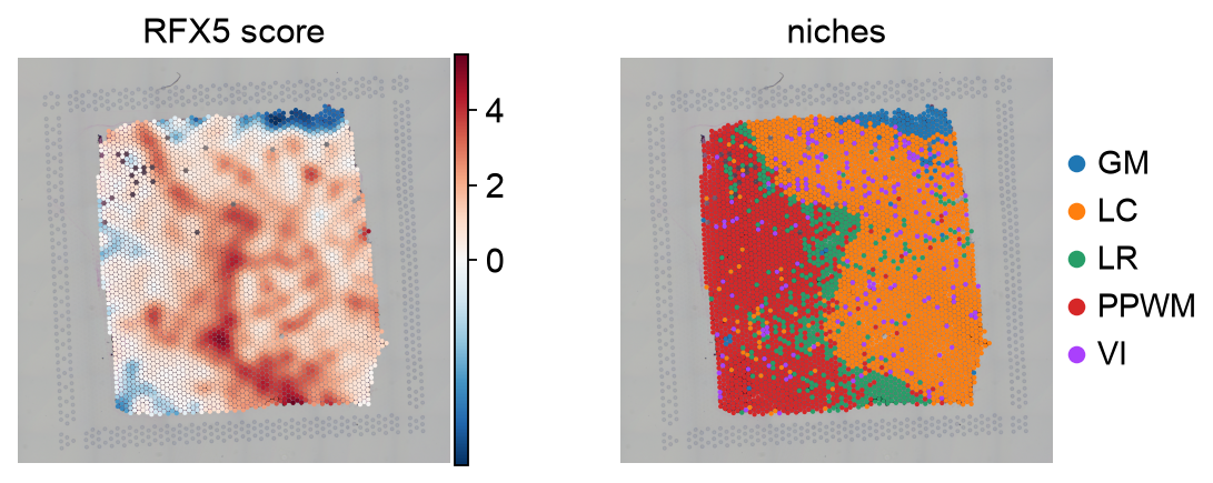
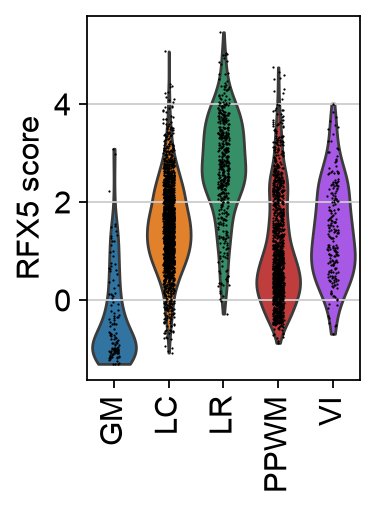
Here, the TF RFX5, a key regulator for antigen-presenting cells, exhibits a strong spatial pattern, showing greater activity in the lesion rim (LR) compared to other areas of the tissue. This aligns with the known fact that these cells are present in this region to engulf cellular debris coming from the lesion core.
This can be compared with the actual expression values of the RFX5 gene.
tf = "RFX5"
sq.pl.spatial_scatter(
    adata, color=[tf, "niches"], size=1.5, title=[f"{tf} expression", "niches"]
)
sc.pl.violin(adata, keys=tf, groupby="niches", rotation=90, ylabel=f"{tf} expression")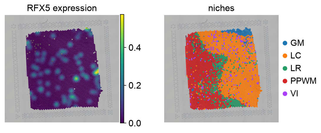
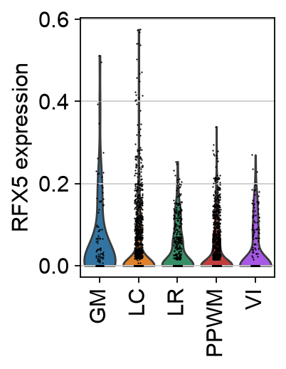
When we look at the expression of the TF RFX5 there is no spatial pattern, as it is randomly expressed across the tissue. TF expression tends to be sporadic and insufficiently informative to determine whether a TF is active in a cell, underscoring the importance of using enrichment scores for interpreting biological data Badia-i-Mompel et al., 2023.
Next, marker TFs for each niche can be identified.
df = dc.tl.rankby_group(
    adata=score, groupby="niches", reference="rest", method="t-test_overestim_var"
)
df = df[df["stat"] > 0.0]
dfThe top 3 TF markers per niche can then be extracted.
n_markers = 3
source_markers = (
    df.groupby("group", observed=False)
    .head(n_markers)
    .drop_duplicates("name")
    .groupby("group", observed=False)["name"]
    .apply(lambda x: list(x))
    .to_dict()
)
source_markers
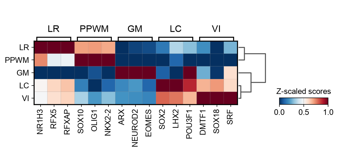
{'GM': ['ARX', 'NEUROD2', 'EOMES'],
'LC': ['SOX2', 'LHX2', 'POU3F1'],
'LR': ['NR1H3', 'RFX5', 'RFXAP'],
'PPWM': ['SOX10', 'OLIG1', 'NKX2-2'],
'VI': ['DMTF1', 'SOX18', 'SRF']}The obtained markers can be plotted
sc.tl.dendrogram(adata=score, groupby="niches")
sc.pl.matrixplot(
    adata=score,
    var_names=source_markers,
    groupby="niches",
    dendrogram=True,
    standard_scale="var",
    colorbar_title="Z-scaled scores",
    cmap="RdBu_r",
)
Individual TFs can be examined by plotting their score distributions.
tf = "OLIG1"
sq.pl.spatial_scatter(
    score,
    color=[tf, "niches"],
    cmap="RdBu_r",
    vcenter=0,
    size=1.5,
    title=[f"{tf} score", "niches"],
)
sc.pl.violin(score, keys=[tf], groupby="niches", rotation=90, ylabel=f"{tf} score")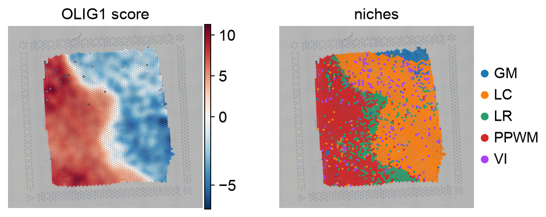
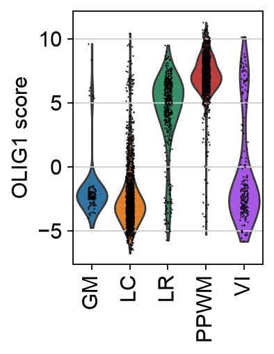
Here, the TF activities for OLIG1 can be observed. OLIG1 is a known marker TF for oligodendrocytes, which are present in the PPWM.
A note on the redundancy between gene sets
Generally, there can be a large overlap between closely related gene sets.
The overlap could be due to gene sets belonging to the same ontology, or describing biological processes that are involved in similar functions.
For example, in this dataset we have seen the gene sets REACTOME_INTERFERON_ALPHA_BETA_SIGNALING and REACTOME_INTERFERON_SIGNALING both being enriched, the former being the specific immune response and the later is the general one.
This overlap impacts the rank of the gene sets in the enrichment results.
It is important to interpret what is the general state of the biological system being studied, in this case it is clear that immune signaling might be happening.
Moreover, it might be beneficial to select tailored gene sets and footprint resources, to reduce the number of possible false positives.
Enrichment frameworks improve biological interpretation by providing testing procedures with different null hypotheses, and including prior knowledge in the computational methods.
See Also
The chapter was mainly adapted from the decoupler tutorials. For further details, we recommend consulting the corresponding vignettes.
Multiple choice questions
Contributors
We gratefully acknowledge the contributions of:
Authors
Soroor Hediyeh-Zadeh
Pau Badia-i-Mompel
Isaac Virshup
Luis Heinzlmeier
Reviewers
Lukas Heumos
Anastasia Litinetskaya
- Subramanian, A., Tamayo, P., Mootha, V. K., Mukherjee, S., Ebert, B. L., Gillette, M. A., Paulovich, A., Pomeroy, S. L., Golub, T. R., Lander, E. S., & others. (2005). Gene set enrichment analysis: a knowledge-based approach for interpreting genome-wide expression profiles. Proceedings of the National Academy of Sciences, 102(43), 15545–15550.
- Liberzon, A., Subramanian, A., Pinchback, R., Thorvaldsdóttir, H., Tamayo, P., & Mesirov, J. P. (2011). Molecular signatures database (MSigDB) 3.0. Bioinformatics, 27(12), 1739–1740.
- Zhang, X., Lan, Y., Xu, J., Quan, F., Zhao, E., Deng, C., Luo, T., Xu, L., Liao, G., Yan, M., & others. (2019). CellMarker: a manually curated resource of cell markers in human and mouse. Nucleic Acids Research, 47(D1), D721–D728.
- Franzén, O., Gan, L.-M., & Björkegren, J. L. (2019). PanglaoDB: a web server for exploration of mouse and human single-cell RNA sequencing data. Database, 2019.
- Szalai, B., & Saez-Rodriguez, J. (2020). Why do pathway methods work better than they should? FEBS Letters, 594(24), 4189–4200.
- Dugourd, A., & Saez-Rodriguez, J. (2019). Footprint-based functional analysis of multiomic data. Current Opinion in Systems Biology, 15, 82–90.
- Schubert, M., Klinger, B., Klünemann, M., Sieber, A., Uhlitz, F., Sauer, S., Garnett, M. J., Blüthgen, N., & Saez-Rodriguez, J. (2018). Perturbation-response genes reveal signaling footprints in cancer gene expression. Nature Communications, 9(1), 1–11.
- Jiang, P., Zhang, Y., Ru, B., Yang, Y., Vu, T., Paul, R., Mirza, A., Altan-Bonnet, G., Liu, L., Ruppin, E., Wakefield, L., & Wucherpfennig, K. W. (2021). Systematic investigation of cytokine signaling activity at the tissue and single-cell levels. Nature Methods, 18(10), 1181–1191.
- Garcia-Alonso, L., Holland, C. H., Ibrahim, M. M., Turei, D., & Saez-Rodriguez, J. (2019). Benchmark and integration of resources for the estimation of human transcription factor activities. Genome Research, 29(8), 1363–1375.
- Squair, J. W., Gautier, M., Kathe, C., Anderson, M. A., James, N. D., Hutson, T. H., Hudelle, R., Qaiser, T., Matson, K. J. E., Barraud, Q., Levine, A. J., La Manno, G., Skinnider, M. A., & Courtine, G. (2021). Confronting false discoveries in single-cell differential expression. Nature Communications, 12(1), 5692.
- Crowell, H. L., Soneson, C., Germain, P.-L., Calini, D., Collin, L., Raposo, C., Malhotra, D., & Robinson, M. D. (2020). muscat detects subpopulation-specific state transitions from multi-sample multi-condition single-cell transcriptomics data. Nature Communications, 11(1), 6077.
- Holland, C. H., Tanevski, J., Perales-Patón, J., Gleixner, J., Kumar, M. P., Mereu, E., Joughin, B. A., Stegle, O., Lauffenburger, D. A., Heyn, H., & others. (2020). Robustness and applicability of transcription factor and pathway analysis tools on single-cell RNA-seq data. Genome Biology, 21(1), 1–19.
- Qoku, A., & Buettner, F. (2022). Encoding Domain Knowledge in Multi-view Latent Variable Models: A Bayesian Approach with Structured Sparsity. arXiv.
- Kunes, R. Z., Walle, T., Nawy, T., & Pe’er, D. (2022). Supervised discovery of interpretable gene programs from single-cell data. bioRxiv.
- Zhang, Y., Ma, Y., Huang, Y., Zhang, Y., Jiang, Q., Zhou, M., & Su, J. (2020). Benchmarking algorithms for pathway activity transformation of single-cell RNA-seq data. Computational and Structural Biotechnology Journal, 18, 2953–2961.