Dimensionality reduction and clustering - Single-cell best practices

Steps

yml

Install conda:
- Before creating the environment, ensure that conda is installed on your system.
Save the yml content:
- Copy the content from the yml tab into a file named environment.yml.
Create the environment:
- Open a terminal or command prompt.
- Run the following command:
```
conda env create -f environment.yml
```
Activate the environment:
- After the environment is created, activate it using:
```
conda activate <environment_name>
```
- Replace <environment_name> with the name specified in the environment.yml file. In the yml file it will look like this:
```
name: <environment_name>
```
Verify the installation:
- Check that the environment was created successfully by running:
```
conda env list
```

chromatin_accessibility.yml

name: chromatin-accessibility
channels:
  - conda-forge
dependencies:
  - conda-forge::ipykernel=7.3.0
  - conda-forge::ipywidgets=8.1.9
  - conda-forge::python=3.13.15
  - conda-forge::scanpy=1.12.4
  - pip
  - pip:
      - lamindb==2.10.0
      - macs3==3.0.5
      - muon==0.1.9
      - snapatac2==2.10.0

This book uses lamindb to store, share, and load datasets and notebooks using the theislab/sc-best-practices instance. We acknowledge free hosting from Lamin Labs.

Install lamindb
- Install the lamindb Python package:
```
pip install lamindb
```
Optionally create a lamin account
- Sign up and log in following the instructions
Verify your setup
- Run the lamin connect command:
```
import lamindb as ln

ln.Artifact.connect("theislab/sc-best-practices").df()
```
You should now see up to 100 of the stored datasets.
Accessing datasets (Artifacts)
- Search for the datasets on the Artifacts page
- Load an Artifact and the corresponding object:
```
import lamindb as ln
af = ln.Artifact.connect("theislab/sc-best-practices").get(key="key_of_dataset", is_latest=True)
obj = af.load()
```
The object is now accessible in memory and is ready for analysis. Adapt the lamindb.Artifact.connect("theislab/sc-best-practices").get("SOMEIDXXXX") suffix to get respective versions.
Accessing notebooks (Transforms)
- Search for the notebook on the Transforms page
- Load the notebook:
```
lamin load <notebook url>
```
which will download the notebook to the current working directory. Analogously to Artifacts, you can adapt the suffix ID to get older versions.

Motivation¶

Unlike genes in scRNA-seq data, scATAC-seq data have no predefined features. Peaks called on all cells miss regions that are only accessible in rare cell types, while peaks called per cluster require clusters in the first place. We therefore count fragments in fixed 500 bp tiles across the genome, which cluster cells as well as peaks do Luo et al., 2024, and call peaks per cell type in the next chapter. We keep counts instead of binarizing them, since the number of fragments in a region carries information Martens et al., 2024, and SnapATAC2 counts the two insertions of a fragment only once if both fall into the same tile Miao & Kim, 2024.

import logging

import lamindb as ln
import scanpy as sc
import snapatac2 as snap

for name in ("kaleido", "choreographer"):
    logging.getLogger(name).setLevel(logging.WARNING)
sc.set_figure_params(dpi=80, facecolor="white", frameon=False)

ln.connect("theislab/sc-best-practices")

ln.track("x9Pv2jyr9s04")

→ connected lamindb: theislab/sc-best-practices

→ loaded Transform('x9Pv2jyr9s040000', key='dimensionality_reduction_clustering.ipynb'), started new Run('kEvPN62vBb8JKGqD') at 2026-09-29 15:27:38 UTC

→ notebook imports: lamindb-core==2.10.0 scanpy==1.12.4 snapatac2==2.10.0

We load the cells that passed quality control, which already contain the tile matrix.

adata = ln.Artifact.get(
    key="chromatin_accessibility/pbmc10k_quality_control.h5ad"
).load()
adata

AnnData object with n_obs × n_vars = 9255 × 6062095
    obs: 'n_fragment', 'frac_dup', 'frac_mito', 'tsse', 'doublet_probability', 'doublet_score'
    var: 'count', 'selected'
    uns: 'TSS_profile', 'doublet_rate', 'frac_overlap_TSS', 'frag_size_distr', 'library_tsse', 'reference_sequences', 'scrublet_sim_doublet_score'
    obsm: 'fragment_paired'
    layers: None (.X)

Dimensionality reduction¶

Of the 6 million tiles, we selected the 250,000 most informative ones during quality control, close to the 200,000 features with which SnapATAC2 performed best in the benchmark Luo et al., 2024. SnapATAC2’s spectral embedding computes the eigenvectors of the cosine similarity between cells without building the full similarity matrix, which makes it scale to millions of cells Zhang et al., 2024. It also separated cell types better than latent semantic indexing (LSI), whose components remain correlated with the number of fragments per cell Luo et al., 2024.

snap.tl.spectral(adata)

Clustering¶

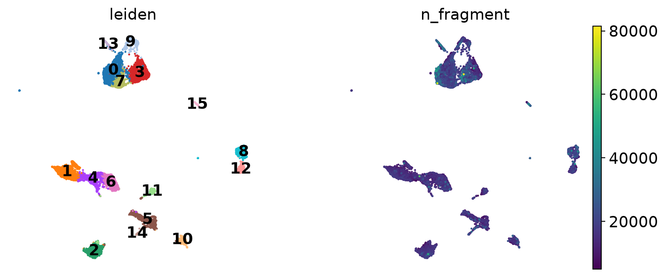
We cluster the cells with the Leiden algorithm on a nearest neighbor graph of the spectral embedding and visualize them with UMAP. Coloring by the number of fragments checks that the embedding is not driven by sequencing depth.

snap.pp.knn(adata)
snap.tl.leiden(adata)
snap.tl.umap(adata)

/home/lheumos/miniforge3/envs/chromatin-accessibility/lib/python3.13/site-packages/umap/umap_.py:1952: UserWarning: n_jobs value 1 overridden to 1 by setting random_state. Use no seed for parallelism.
  warn(

sc.pl.umap(adata, color=["leiden", "n_fragment"], legend_loc="on data")

... storing 'leiden' as categorical

Cell type annotation¶

We annotate the clusters through the accessibility of marker genes. SnapATAC2 estimates the activity of a gene from the insertions in its gene body and the 2 kb upstream of it, which approximated gene expression best among the tools in the benchmark Luo et al., 2024. Accessibility of a gene does not imply that it is transcribed, so a cell type should be supported by several markers.

annotation = ln.Artifact.get(
    key="chromatin_accessibility/gencode_v41_GRCh38.gff3.gz"
).cache()
gene_activity = snap.pp.make_gene_matrix(adata, annotation)
sc.pp.normalize_total(gene_activity)
sc.pp.log1p(gene_activity)

markers = {
    "CD14+ Mono": ["FCN1", "TREM1", "FPR1"],
    "CD16+ Mono": ["TCF7L2", "LYN"],
    "cDC2": ["FCER1A", "CLEC10A"],
    "pDC": ["PTPRS", "KCNN3", "TCF4"],
    "B": ["MS4A1", "PAX5", "CD79A"],
    "Naive B": ["TCL1A", "IGHD"],
    "Memory B": ["TNFRSF13B"],
    "NK": ["GNLY", "KLRD1", "CD160"],
    "MAIT": ["SLC4A10", "KLRB1"],
    "T": ["CD3E", "BCL11B"],
    "CD8+ T": ["CD8A", "CD8B"],
    "Naive T": ["LEF1", "CCR7", "BACH2"],
    "Effector T": ["CCL5", "GZMK"],
}
sc.pl.dotplot(
    gene_activity,
    markers,
    groupby="leiden",
    standard_scale="var",
    colorbar_title="Scaled gene activity",
)

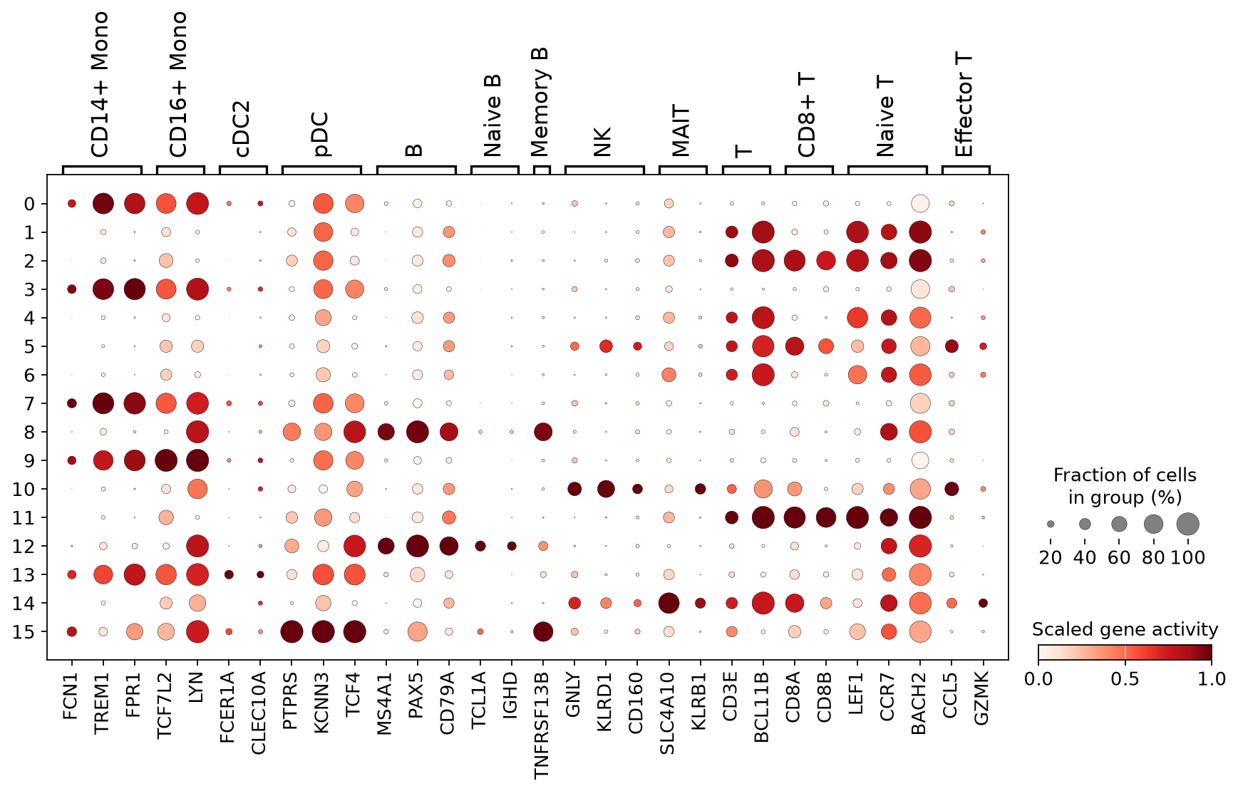
Clusters 0, 3, 7 and 9 are monocytes, of which cluster 9 are CD16+ monocytes with the highest activity of TCF7L2, and cluster 13 are cDC2 with FCER1A and CLEC10A. Cluster 15 are pDCs. The B cells split into naive B cells with TCL1A and IGHD in cluster 12 and memory B cells with TNFRSF13B in cluster 8. Cluster 10 are NK cells and cluster 14 MAIT cells. All other clusters are T cells with CD3E and BCL11B. Clusters 2 and 11 are naive CD8+ T cells, cluster 5 effector CD8+ T cells with CCL5 and GZMK, and clusters 1, 4 and 6 CD4+ T cells, which we keep together because these markers do not clearly separate naive from memory CD4+ T cells.

cell_types = {
    "0": "CD14+ Mono",
    "1": "CD4+ T",
    "2": "Naive CD8+ T",
    "3": "CD14+ Mono",
    "4": "CD4+ T",
    "5": "Effector CD8+ T",
    "6": "CD4+ T",
    "7": "CD14+ Mono",
    "8": "Memory B",
    "9": "CD16+ Mono",
    "10": "NK",
    "11": "Naive CD8+ T",
    "12": "Naive B",
    "13": "cDC2",
    "14": "MAIT",
    "15": "pDC",
}
adata.obs["cell_type"] = adata.obs["leiden"].map(cell_types).astype("category")
sc.pl.umap(adata, color="cell_type")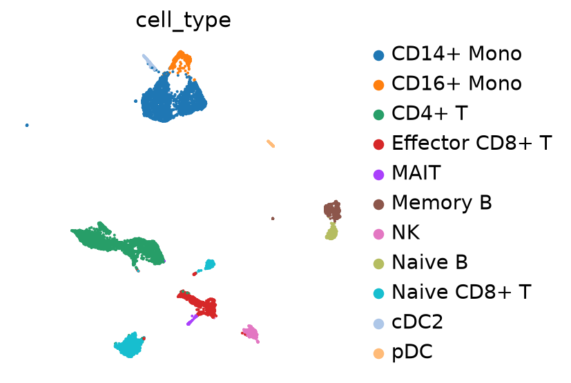

We store the annotated cells for peak calling.

ln.Artifact.from_anndata(
    adata,
    key="chromatin_accessibility/pbmc10k_clustered.h5ad",
    description="PBMC 10k multiome chromatin accessibility after clustering and annotation",
).save()

→ returning artifact with same hash: Artifact(uid='19dwbxDQ04HPT3VL0001', key='chromatin_accessibility/pbmc10k_clustered.h5ad', description='PBMC 10k multiome chromatin accessibility after clustering and annotation', suffix='.h5ad', kind='dataset', otype='AnnData', size=3269556941, hash='ZQsH6oBKvLqDqJDaJabYvF', n_files=None, n_observations=9255, extra_data=None, branch_id=1, created_on_id=1, space_id=1, storage_id=1, run_id=166, schema_id=None, created_by_id=2, created_at=2026-09-29 14:46:09 UTC, is_locked=False, version_tag=None, is_latest=True); to track this artifact as an input, use: ln.Artifact.get()

Artifact(uid='19dwbxDQ04HPT3VL0001', key='chromatin_accessibility/pbmc10k_clustered.h5ad', description='PBMC 10k multiome chromatin accessibility after clustering and annotation', suffix='.h5ad', kind='dataset', otype='AnnData', size=3269556941, hash='ZQsH6oBKvLqDqJDaJabYvF', n_files=None, n_observations=9255, extra_data=None, branch_id=1, created_on_id=1, space_id=1, storage_id=1, run_id=166, schema_id=None, created_by_id=2, created_at=2026-09-29 14:46:09 UTC, is_locked=False, version_tag=None, is_latest=True)

Contributors¶

We gratefully acknowledge the contributions of:

Authors¶

Lukas Heumos

References¶

Luo, S., Germain, P.-L., Robinson, M. D., & von Meyenn, F. (2024). Benchmarking computational methods for single-cell chromatin data analysis. Genome Biology, 25(1), 225. 10.1186/s13059-024-03356-x
Martens, L. D., Fischer, D. S., Yépez, V. A., Theis, F. J., & Gagneur, J. (2024). Modeling fragment counts improves single-cell ATAC-seq analysis. Nature Methods, 21(1), 28–31. 10.1038/s41592-023-02112-6
Miao, Z., & Kim, J. (2024). Uniform quantification of single-nucleus ATAC-seq data with Paired-Insertion Counting (PIC) and a model-based insertion rate estimator. Nature Methods, 21(1), 32–36. 10.1038/s41592-023-02103-7
Zhang, K., Zemke, N. R., Armand, E. J., & Ren, B. (2024). A fast, scalable and versatile tool for analysis of single-cell omics data. Nature Methods, 21(2), 217–227. 10.1038/s41592-023-02139-9