38. Immune Receptor Profiling

38.1. Role IR in cells

Immune Receptors (IR) are the key for the recognition of potential hazardous antigens and toxins invading the body. Those receptors are usually located in the membrane of specialized cells, which recognize harmful content and initiate protective mechanisms. There are different kinds of IRs specialized in the recognition of specific structures of foreign agents:

• Pattern recognition receptors (PRRs): Pathogen-associated molecular patterns (PAMPS)

• Killer activator/inhibitor receptors (KARs/KIRs): Host cells abnormalities

• Complement receptors: Complement proteins

• Fc receptors: Epitope-antibody complex

• Cytokine receptors: Cytokines

• B-cell receptor (BCRs): Epitopes

• T-cell recpetors (TCRs): Linear epitopes bound to the Major Histocompatibility Complex (MHC)

38.2. IRs of the adaptive immune system

In the adaptive immune system, there are two major lineages of lymphocytes with IRs, which are produced in the Thymus and Bone-marrow called T- and B-cells [Cooper and Alder, 2006]. These adaptive immune receptors (AIRs) of both cell lines detect antigens derived from different pathogens and tumor cells. However, they interact with the antigens in different ways: While the B-cell receptor (BCR) directly recognizes soluble or membrane-bound epitopes, the T-cell receptor interacts with linear peptides bound to the surface protein MHC (pMHC), which enables to view inside cells by presenting its content on the cell’s surface. After activation by antigens, B- and T-cells perform various functions such as fighting the pathogen, regulation of the immune response, or forming memory by proliferation.

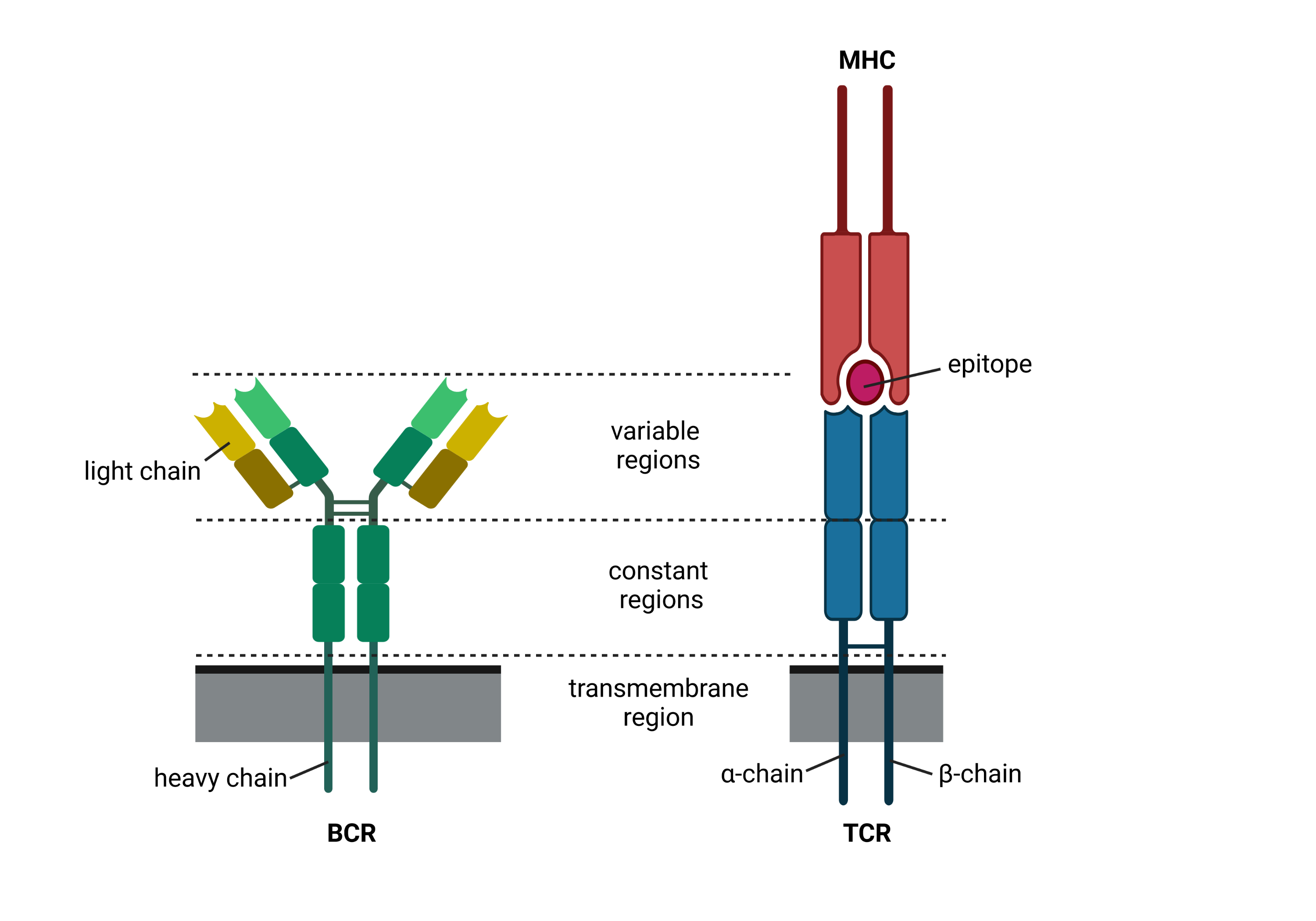
Fig. 38.1 Schematic drawing of the two AIR types. Created with BioRender.com.

38.3. Formation of adaptive immune receptors by V(D)J recombination

The AIR is a protein complex consisting of two chains. Depending on the T cell type, these chains are either called α- and β- or γ- and δ-chain. Similarly, the BCR chains are called heavy and light chain (subtypes: κ and λ). While the α-, γ-, κ-, and λ-chains are formed by their respective V- and J-genes, the remaining chains additionally include their D-gene. For simplicity, we will therefore refer to VJ and VDJ chains throughout this book.

Adaptive IRs lines are highly polymorphic in order to capture the immense space of antigens, i.e., there exists an immense variety of different TCR and BCR sequences. The amount of different TCRs have been estimated at 10²⁰ in total, while a human individual harbors 10⁷ different sequences [Zarnitsyna et al., 2013]. Similarly, there naturally occur up to 10¹⁸ different BCRs [Briney et al., 2019]. The collection of all receptors forms the AIR repertoire of an individual.

The sequence diversity is introduced by the V(D)J recombination mechanism:

• Combinatorial diversity is introduced by the combination of different V-, (D-,) and J-genes in addition to the combination of different VJ and VDJ chains.

• Junctional diversity is achieved by insertion of nucleotides at the gene interfaces.

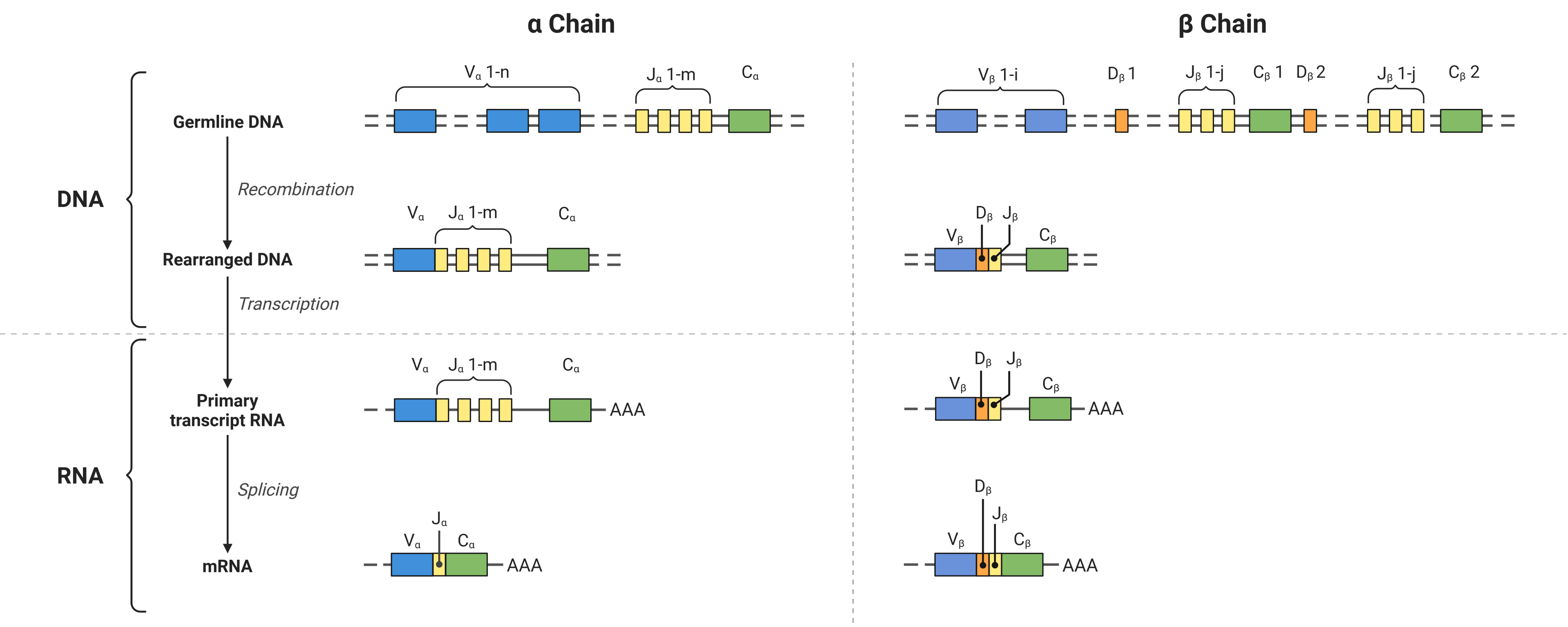
Fig. 38.2 VDJ recombination at the example of an αβ-TCR. Created with BioRender.com.

Additionally, mutations occur at the BCR binding sites in a process called Somatic Hypermutation for affinity maturation during rapid cell proliferation.

In the resulting AIRs, three regions of high variability - the Complementary Determining Regions (CDRs) 1-3 - were detected per chain, where the AIR interacts with its target. The CDR1 and CDR2 are encoded by the V-gene. However, the CDR3 spans over the intersection of V-, (D-,) and J-genes and is therefore the most diverse element of the AIR. Therefore, it is often assumed that the specificity of an AIR is determined mainly by its CDR3 region of the more diverse VDJ chain.

38.4. VDJ-sequencing

38.4.1. Cell isolation

Before quantifying the single-cell data, the cells of interest should be targeted and isolated. Common options include:

• Fluorescence Activated Cell Sorting (FACS) is a method based on flow cytometry with the power to label the cells of interest based on fluorescent probes over the raw cell suspension. A cell suspension is carried by a rapidly flowing stream of liquid. This stream of cells is broken up into individual droplets through a vibrating mechanism. Just before the stream breaks into droplets, the flow passes through a fluorescence measuring station where the fluorescence signal of every cell is measured. The droplets can be further charged for further separations.

• Magnetic-Activated Cell Sorting (MACS) can use antibodies, enzymes, lectins, or strepavidins attached to a magnetic bead to label the target cells. Once the cells are labeled from the raw suspension, a magnetic field is applied to attract the magnetic beads and discard the remaining cells from the suspensions. The targeted cells are collected once the magnetic field is turned off. One advantage of this method is the capacity to collect targeted cells with no specific markers to be labeled, in that case, a cocktail of markers is used to label the untargeted cells, and the cells of interests are collected by washing them out once the magnetic field captures the untargeted cells conjugated to a magnetic bead.

• Laser Capture Microdissection (LCM) has the power to extract cell populations or single cells from microscope preparations without detriment of the surrounding tissue. The components to perform LCM includes a reverse micrsocope, a laser control unit, a microscope joy stick to plate stabilization, a CCD camera, and a color monitor. The idea behind LCM consists on labelling cells by visual detection of morphological characteristics of target cells, the plate is immobilized and the laser pulse melts the thin thermoplastic film removing the cells or cells of interest without any damage to the surrounding tissue.

• Microfluidics is a versatile method able to work with small quantities of raw suspension even at the order of nanoliters. There are different kinds of microfluidic approaches including cell-affinity chromatographu based microfluidics, physical characteristics of cell based microfluidics, immunomagnetics beads based microfluidics, and separation by dielectric properties of some cell-types based microfluifdics. The most used microfluidics based method is the chromatographic separation using a chip assay as stationary phase which is modified to include the necessary antibodies to capture the target cells in the mobile phase. After the buffer flows off from the chip, a solution is used to separate the cells attached to the antibodies to collect them for further analysis [Hu et al., 2016].

38.4.2. Immune receptor sequencing

A common approach to discern V(D)J chains from single-cell isolations consist on computational reconstructions of different chains sequences based on full-length single-cell RNA sequencing, being Smart-seq2, a 5’-end RNA template based protocol, one of the widest implemented. Regarding computational methods, TRAPeS, TraCer, and VDJPuzzle are usually used to reconstruct TCR sequences based on scRNA-seq data, whereas BALDR [Upadhyay et al., 2018], BASIC [Canzar et al., 2016] and BraCer [Lindeman et al., 2018] were shown to robustly recover BCR sequences. However, they are prone to ignore the whole landscape of recombinatorial products and alternative splicing products in V(D)J region. Some alternatives have rise to deal with this problematic, RAGE-seq for example was developed to capture specific TCR and BCR fragments based on PCR templates designed for immune receptor sequencing and use long-read Oxford Nanopore to capture the whole sequence, whereas the rest of the cDNA is processed based on short-reads protocols provided by, for example, Illumina [Singh et al., 2019].

38.5. AIR repertoire analysis

VDJ-sequencing provides us with the nucleotide and thereby also the protein sequence of the AIR paired for both chains, from which the V-, (D-,) J-, and C-gene is determined in addition to the CDR3 sequence. Overall, the AIR sequence determines the specificity of the individual B- and T-cell. Therefore, the information obtained by VDJ-sequencing provides us with an indicator of the cells’ functionality, which is directly coupled to the AIRs target antigen. This enables us to use the AIR information in three major ways:

• Phenotyping: We can group immune cells by identifying cells with the same or similar AIR, which share the same specificity. Having these groups, we can now observe, how disease-specific cells react under different conditions (e.g. transcriptomic change upon stimulation), whether immune cells have proliferated, or how the diversity of an immune repertoire changes upon after an immune response.

• Sequence Analysis: Having identified groups of AIRs (e.g. a reactive cluster detected in other modalities), we can extract properties of their sequence, such as V-, D-, and J-, gene usage or enriched sequence motifs, that are related to specific diseases or therapies.

• Specificity-Inference: Last, we can use the sequence to match AIRs to their target antigen via database queries, sequence distances, or predictors. This directly identifies cells reactive to specific infectious diseases, tumors, or self-antigens.

38.6. Dataset

To showcase different approaches for preprocessing and analysis of IRs, we will use the dataset published by the Haniffa Lab [Stephenson et al., 2021], which contains transcriptome sequencing for over 750,000 Peripheral Blood Mononuclear Cells (PBMC) from 130 patients in the context of Severe Acute Respiratory Syndrome Coronavirus 2 (SARS-CoV-2).

It consists of patients from three sources (Newcastle, Cambridge, and London) with different degrees of severity (asymptomatic, mild, moderate, severe, and critical) as well as negative controls (healthy, other severe respiratory illnesses, and healthy with Intravenous Liposaccharide to mimic systemic inflammatory response). Additional, patient-level information such as age, gender, and smoker status are provided.

The dataset was chosen as an example of a large-scale single cell dataset including VDJ-Sequencing, that is well known to the community. It contains over 150,000 B-Cells and 200,000 T-Cells with IR annotation, that we will regard in this analysis tutorial.

To download the data please run the following commands:

path_data = "data/"
path_bcr_input = f"{path_data}/BCR_00_read_aligned.csv"
path_tcr_input = f"{path_data}/TCR_00_read_aligned.tsv"

! wget -O $path_bcr_input -nc https://figshare.com/ndownloader/files/35574338
! wget -O $path_tcr_input -nc https://figshare.com/ndownloader/files/35574539

--2022-06-07 18:30:52--  https://figshare.com/ndownloader/files/35574338
Resolving figshare.com (figshare.com)... 54.72.163.193, 52.50.42.102, 2a05:d018:1f4:d000:7421:2135:71b2:6a10, ...
Connecting to figshare.com (figshare.com)|54.72.163.193|:443... connected.
HTTP request sent, awaiting response... 302 Found
Location: https://s3-eu-west-1.amazonaws.com/pfigshare-u-files/35574338/bcr_cellranger.csv?X-Amz-Algorithm=AWS4-HMAC-SHA256&X-Amz-Credential=AKIAIYCQYOYV5JSSROOA/20220607/eu-west-1/s3/aws4_request&X-Amz-Date=20220607T163052Z&X-Amz-Expires=10&X-Amz-SignedHeaders=host&X-Amz-Signature=b18cb63ca03820e07cb8b3d9375466ca6405e655822269f5ae36d7449a28b810 [following]
--2022-06-07 18:30:52--  https://s3-eu-west-1.amazonaws.com/pfigshare-u-files/35574338/bcr_cellranger.csv?X-Amz-Algorithm=AWS4-HMAC-SHA256&X-Amz-Credential=AKIAIYCQYOYV5JSSROOA/20220607/eu-west-1/s3/aws4_request&X-Amz-Date=20220607T163052Z&X-Amz-Expires=10&X-Amz-SignedHeaders=host&X-Amz-Signature=b18cb63ca03820e07cb8b3d9375466ca6405e655822269f5ae36d7449a28b810
Resolving s3-eu-west-1.amazonaws.com (s3-eu-west-1.amazonaws.com)... 52.218.62.171
Connecting to s3-eu-west-1.amazonaws.com (s3-eu-west-1.amazonaws.com)|52.218.62.171|:443... connected.
HTTP request sent, awaiting response... 200 OK
Length: 84451806 (81M) [text/csv]
Saving to: ‘data//BCR_00_read_aligned.csv’

100%[======================================>] 84,451,806  39.1MB/s   in 2.1s   

2022-06-07 18:30:54 (39.1 MB/s) - ‘data//BCR_00_read_aligned.csv’ saved [84451806/84451806]

--2022-06-07 18:30:55--  https://figshare.com/ndownloader/files/35574539
Resolving figshare.com (figshare.com)... 54.72.163.193, 52.50.42.102, 2a05:d018:1f4:d000:7421:2135:71b2:6a10, ...
Connecting to figshare.com (figshare.com)|54.72.163.193|:443... connected.
HTTP request sent, awaiting response... 302 Found
Location: https://s3-eu-west-1.amazonaws.com/pfigshare-u-files/35574539/TCR_mergedUpdated.tsv?X-Amz-Algorithm=AWS4-HMAC-SHA256&X-Amz-Credential=AKIAIYCQYOYV5JSSROOA/20220607/eu-west-1/s3/aws4_request&X-Amz-Date=20220607T163055Z&X-Amz-Expires=10&X-Amz-SignedHeaders=host&X-Amz-Signature=141ab989ae794394fb6c441d50c0ea6771f96a8d048a8a4c400c10dba267b97c [following]
--2022-06-07 18:30:55--  https://s3-eu-west-1.amazonaws.com/pfigshare-u-files/35574539/TCR_mergedUpdated.tsv?X-Amz-Algorithm=AWS4-HMAC-SHA256&X-Amz-Credential=AKIAIYCQYOYV5JSSROOA/20220607/eu-west-1/s3/aws4_request&X-Amz-Date=20220607T163055Z&X-Amz-Expires=10&X-Amz-SignedHeaders=host&X-Amz-Signature=141ab989ae794394fb6c441d50c0ea6771f96a8d048a8a4c400c10dba267b97c
Resolving s3-eu-west-1.amazonaws.com (s3-eu-west-1.amazonaws.com)... 52.218.62.171
Connecting to s3-eu-west-1.amazonaws.com (s3-eu-west-1.amazonaws.com)|52.218.62.171|:443... connected.
HTTP request sent, awaiting response... 200 OK
Length: 247085830 (236M) [text/tab-separated-values]
Saving to: ‘data//TCR_00_read_aligned.tsv’

100%[======================================>] 247,085,830 42.4MB/s   in 5.8s   

2022-06-07 18:31:01 (40.9 MB/s) - ‘data//TCR_00_read_aligned.tsv’ saved [247085830/247085830]

38.7. Load data

In this tutorial we will mainly use two python packages for loading, cell-level ordering, and visualiation:

• Scanpy: general package for single cell analysis (theislab/scanpy, [Wolf et al., 2018])

• Scirpy: scanpy extension for immune receptor analysis (scverse/scirpy, [Sturm et al., 2020])

Here, we only showcase IR analysis with Scirpy. However, there exist several tools with similar functionality such as immunarch(R, [ImmunoMind Team, 2019]), scRepertoire (R, [Borcherding et al., 2020]), and dandelion (R, [Stephenson et al., 2021]), and Platypus (R, [Yermanos et al., 2021]) reviewed in [Valkiers et al., 2022].

Warning

Scirpy changed the format of its datastructure with v0.13. While the overall anlaysis workflow has not changed, some outputs shown in this chapter might not be accurate anymore.

See the scirpy release notes for more details about this change. Until we update this chapter, please also refer to the official scirpy documentation.

import warnings

warnings.filterwarnings(
    "ignore",
    ".*IProgress not found*",
)
warnings.simplefilter(action="ignore", category=FutureWarning)

import scanpy as sc
import scirpy as ir

import pandas as pd

warnings.simplefilter(action="ignore", category=pd.errors.DtypeWarning)

Let’s set the input and output paths of our data.

path_bcr_out = f"{path_data}/BCR_01_preprocessed.h5ad"

path_tcr_csv = f"{path_data}/TCR_00_read_aligned.csv"
path_tcr_out = f"{path_data}/TCR_01_preprocessed.h5ad"

38.7.1. Raw data

We begin by with viewing the raw output of the cell ranger pipeline for a better understanding of the data we are working with. We will load the filtered_contig_annotations.csv" file to view its content. Each row will represent one measurement of a sequence.

df_bcr_raw = pd.read_csv(path_bcr_input, index_col=0)

# The column 'productive' contains mixed data types which are not compatible with downstream tools.
# We correct them by casting them to strings.
df_bcr_raw["productive"] = df_bcr_raw["productive"].astype(str)
print(f"Total measurements: {len(df_bcr_raw)}")
df_bcr_raw.head(5)

Total measurements: 373670

	barcode	is_cell	contig_id	high_confidence	length	chain	v_gene	d_gene	j_gene	c_gene	full_length	productive	cdr3	cdr3_nt	reads	umis	raw_clonotype_id	raw_consensus_id	patient_id	newBarcode
0	AAACCTGAGCGATATA-MH9143270	True	AAACCTGAGCGATATA-MH9143270_contig_1	True	646	IGL	IGLV1-44	None	IGLJ1	IGLC2	True	True	CAAWDDSLSASYVF	TGTGCAGCATGGGATGACAGCCTGAGTGCCTCTTATGTCTTC	154	14	clonotype9	clonotype9_consensus_2	COVID-002	NaN
1	AAACCTGAGCGATATA-MH9143270	True	AAACCTGAGCGATATA-MH9143270_contig_2	True	579	IGH	IGHV3-33	IGHD3-3	IGHJ4	IGHM	True	True	CARDNRVYYDFWSGYPDYW	TGTGCGAGAGACAACCGAGTCTATTACGATTTTTGGAGTGGTTATC...	144	13	clonotype9	clonotype9_consensus_1	COVID-002	NaN
2	AAACCTGTCTACCAGA-MH9143270	True	AAACCTGTCTACCAGA-MH9143270_contig_1	True	574	IGH	IGHV1-69D	IGHD2-15	IGHJ5	IGHM	True	True	CARDRRSAYCSGGSCWGGDWFDPW	TGTGCGAGAGATCGTCGTTCAGCTTATTGTAGTGGTGGTAGCTGCT...	564	42	clonotype10	clonotype10_consensus_1	COVID-002	NaN
3	AAACCTGTCTACCAGA-MH9143270	True	AAACCTGTCTACCAGA-MH9143270_contig_2	True	744	IGL	IGLV1-51	None	IGLJ3	IGLC3	True	False	CGTWDSSLSAWVF	TGCGGAACATGGGATAGCAGCCTGAGTGCTTGGGTGTTC	188	21	clonotype10	None	COVID-002	NaN
4	AAACGGGCATTTGCTT-MH9143270	True	AAACGGGCATTTGCTT-MH9143270_contig_1	True	565	IGH	IGHV3-33	None	IGHJ4	IGHM	True	True	CANPTRPYSSSWWYFDYW	TGTGCGAACCCCACCCGTCCATATAGCAGCAGCTGGTGGTACTTTG...	234	20	clonotype11	clonotype11_consensus_1	COVID-002	NaN

The Table contains the following entries, that will be relevant for our preprocessing or analysis. A more detailed explanation of Cell Ranger specific entries can be found here (https://support.10xgenomics.com/single-cell-vdj/software/pipelines/latest/output/annotation). In other data formats entries (e.g. AIRR) will have similar, deviating names, however the underlying information remains similar.

• barcode: tag of the cell the contig was measured from

• is_cell: indicates whether the barcode is associated with a cell

• high_confidence: confidence of the measurement being a IR

• chain: chain of the IR (e.g. TRA: T Cell Receptor α-chain, IGH: Immuneglobulin Heavy chain)

• {v,d,j,c}_gene: gene used to form the specific segment of the IR

• full_length: whether the full IR was captured (see below)

• productive: whether the IR is productive (see below)

• cdr3{_nt}: {Nucleotide} sequence of the CDR3 of the IR chain

• patient_id: ID indicating the different patients

38.7.2. Productive AIRs

Even though we can detect the AIR sequence, it might not be productive, i.e., it might not form a valid AIR. Sequences, which do not result in functional AIRs, are therefore flagged as non-productive. These are usually ignored, when loading data by tools such as Scirpy, and not used for any downstream analysis. Productive Immune receptors are defined by 10x Genomics here as:

• Sequences spanning over from a V gene to a J-gene

• Having a start codon in the leading region

• Containing a CDR3 in the frame of the start codon.

• Do not contain a stop codon within the V-J span

Example 1: Sequences not spanning over a full IR (V to J gene) as indicated by the full_length column. You can find missing gene annotation here especially for V and J genes.

columns = [
    "barcode",
    "v_gene",
    "d_gene",
    "c_gene",
    "j_gene",
    "productive",
    "full_length",
]
df_bcr_raw[~df_bcr_raw["full_length"]][columns].head()

	barcode	v_gene	d_gene	c_gene	j_gene	productive	full_length
34	AACTCCCCAAGTACCT-MH9143270	None	None	IGLC3	IGLJ5	False	False
38	AACTCTTCAGATCGGA-MH9143270	IGKV1-39	None	IGKC	None	False	False
43	AACTGGTCAGGGAGAG-MH9143270	IGLV4-3	None	IGLC2	None	False	False
65	ACACCAAGTCGATTGT-MH9143270	None	IGHD5-12	IGHD	IGHJ4	False	False
76	ACATCAGCATACTACG-MH9143270	None	IGHD3-3	IGHD	IGHJ6	False	False

Example 2: Contigs express full length but there is not identifieable CDR3.

columns += ["cdr3", "cdr3_nt"]
df_bcr_raw[(df_bcr_raw["productive"] == "False") & (df_bcr_raw["full_length"])][
    columns
].head(5)

	barcode	v_gene	d_gene	c_gene	j_gene	productive	full_length	cdr3	cdr3_nt
3	AAACCTGTCTACCAGA-MH9143270	IGLV1-51	None	IGLC3	IGLJ3	False	True	CGTWDSSLSAWVF	TGCGGAACATGGGATAGCAGCCTGAGTGCTTGGGTGTTC
13	AAAGCAAGTCGAAAGC-MH9143270	IGHV5-51	IGHD2-15	IGHD	IGHJ4	False	True	None	None
23	AACGTTGAGCTGCGAA-MH9143270	IGHV3-30	None	IGHM	IGHJ4	False	True	CESGRATITMIVVTDLDYW	TGCGAAAGCGGGCGGGCTACGATTACTATGATAGTAGTGACTGACC...
27	AACTCAGTCAAAGTAG-MH9143270	IGHV3-23	IGHD3-16	IGHD	IGHJ4	False	True	CAKAWIGLDSEIYYDYIWGSYRIDFDYW	TGTGCGAAAGCTTGGATCGGACTCGACTCCGAGATTTATTATGATT...
30	AACTCCCAGGTGCACA-MH9143270	IGKV6-21	None	IGKC	IGKJ3	False	True	None	None

We will now load the TCR data and convert it from tab-separated format to comma-separated format for later use. Since barcodes overlap between multiple samples within the dataset, we further copy the unique CellID as barcode annotation. This data also contains annotation on patient-level (e.g. age, outcome, …) and cell-level annotation (cell type) in addition to the contig annotations previously discussed.

df_tcr_raw = pd.read_csv(path_tcr_input, sep="\t")
df_tcr_raw["barcode"] = df_tcr_raw.pop("CellID")
df_tcr_raw.to_csv(path_tcr_csv)
print(f"Total measurements: {len(df_tcr_raw)}")
df_tcr_raw.head()

Total measurements: 547630

	Centre	barcode	is_cell	contig_id	high_confidence	length	chain	v_gene	d_gene	j_gene	...	Days_from_onset	time_after_LPS	Worst_Clinical_Status	Outcome	leiden	consensus	initial_clustering	study_id	AgeRange	Age
0	Newcastle	AAACCTGAGAAACCTA-MH9179824	True	AAACCTGAGAAACCTA-1_contig_2	True	512	TRB	TRBV5-1	None	TRBJ2-3	...	8	NaN	Moderate	Home	26	CD8	CD8	COVID-014	(50, 59]	54
1	Newcastle	AAACCTGAGAAACCTA-MH9179824	True	AAACCTGAGAAACCTA-1_contig_1	True	573	TRA	TRAV8-4	None	TRAJ31	...	8	NaN	Moderate	Home	26	CD8	CD8	COVID-014	(50, 59]	54
2	Newcastle	AAACCTGAGAACAATC-MH9143324	True	AAACCTGAGAACAATC-1_contig_1	True	635	TRB	TRBV19	None	TRBJ1-5	...	16	NaN	Moderate	Home	25	gdT	gdT	COVID-029	(20, 29]	26
3	Newcastle	AAACCTGAGAACTCGG-MH8919329	True	AAACCTGAGAACTCGG-1_contig_1	True	499	TRA	TRAV34	None	TRAJ30	...	5	NaN	Death	Death	23	Treg	Treg	COVID-045	(70, 79]	77
4	Newcastle	AAACCTGAGAACTCGG-MH8919329	True	AAACCTGAGAACTCGG-1_contig_2	True	496	TRB	TRBV5-1	None	TRBJ2-5	...	5	NaN	Death	Death	23	Treg	Treg	COVID-045	(70, 79]	77

5 rows × 47 columns

We will find that this data already has been processed: All contigs are of full length and represent a productive IR.

df_tcr_raw["full_length"].value_counts()

True    547630
Name: full_length, dtype: int64

df_tcr_raw["productive"].value_counts()

True    547630
Name: productive, dtype: int64

38.8. Cell-Aligned Data

In order to perform analysis on cell level, we next need to align IR information previously sorted by contig to a cell based format via the cell barcode. Note that usually many contigs map to the same cell, since every IR consists of VJ and VDJ chain. Also, it has been shown, that a cell can express multiple IRs [Schuldt and Binstadt, 2019].

We will utilize the Python package Scirpy, that performs the cell-alignment automatically, when reading various TCR information from various formats:

adata_tcr = ir.io.read_10x_vdj(path_tcr_csv)
print(f"Amount cells: {len(adata_tcr)}")

WARNING: Non-standard locus name ignored: Multi 
Amount cells: 280045

The IR information will be stored sorted in adata_tcr.obs as a Pandas DataFrame with the index representing an individual cell. The DataFrame contains the following columns:

• has_ir: indicates whether an IR was detected

• multi_chain: indicates whether more than 2 IRs were detected

• extra_chains: list of additional chains if multi_chain is true

The contig data we observed in the raw data is stored as well. It is stored as separate columns for the two chains (VJ and VDJ) with up to 2 contigs per chain for each cell:

• IR_V{D}J_{1,2}_locus

• IR_V{D}J_{1,2}_productive

• IR_V{D}J_{1,2}_{v,d,j,c}_call

• IR_V{D}J_{1,2}_junction{_aa}

adata_tcr.obs.head(5)

	is_cell	high_confidence	multi_chain	extra_chains	IR_VJ_1_c_call	IR_VJ_2_c_call	IR_VDJ_1_c_call	IR_VDJ_2_c_call	IR_VJ_1_consensus_count	IR_VJ_2_consensus_count	...	IR_VDJ_2_locus	IR_VJ_1_productive	IR_VJ_2_productive	IR_VDJ_1_productive	IR_VDJ_2_productive	IR_VJ_1_v_call	IR_VJ_2_v_call	IR_VDJ_1_v_call	IR_VDJ_2_v_call	has_ir
cell_id
AAACCTGAGAAACCTA-MH9179824	True	True	False	[]	TRAC	NaN	TRBC2	NaN	960.0	NaN	...	NaN	True	None	True	None	TRAV8-4	NaN	TRBV5-1	NaN	True
AAACCTGAGAACAATC-MH9143324	True	True	False	[]	NaN	NaN	TRBC1	NaN	NaN	NaN	...	NaN	None	None	True	None	NaN	NaN	TRBV19	NaN	True
AAACCTGAGAACTCGG-MH8919329	True	True	False	[]	TRAC	NaN	TRBC2	NaN	5122.0	NaN	...	NaN	True	None	True	None	TRAV34	NaN	TRBV5-1	NaN	True
AAACCTGAGAAGCCCA-MH9143373	True	True	False	[]	TRAC	NaN	NaN	NaN	25914.0	NaN	...	NaN	True	None	None	None	TRAV16	NaN	NaN	NaN	True
AAACCTGAGAAGGACA-MH9143274	True	True	False	[]	TRAC	NaN	TRBC2	NaN	3212.0	NaN	...	NaN	True	None	True	None	TRAV8-1	NaN	TRBV7-6	NaN	True

5 rows × 45 columns

Notice, that the patient-level information is not automatically added here. Let’s add them by loading the raw data, alligning them on a cell level and indexing them by their barcode.

patient_information = [
    "barcode",
    "Centre",
    "Sample",
    "patient_id",
    "Collection_Day",
    "Sex",
    "Swab_result",
    "Status",
    "Smoker",
    "Status_on_day_collection",
    "Status_on_day_collection_summary",
    "Days_from_onset",
    "time_after_LPS",
    "Worst_Clinical_Status",
    "Outcome",
    "initial_clustering",
    "study_id",
    "AgeRange",
    "Age",
]
df_patient = df_tcr_raw[patient_information].copy()
df_patient["Days_from_onset"] = df_patient["Days_from_onset"].astype(
    str
)  # mixed type (str, int)
df_patient = df_patient.drop_duplicates().reset_index(drop=True)

# Assigning barcode as index
df_patient.index = df_patient.pop("barcode")
df_patient.index.name = None
df_patient.head()

	Centre	Sample	patient_id	Collection_Day	Sex	Swab_result	Status	Smoker	Status_on_day_collection	Status_on_day_collection_summary	Days_from_onset	time_after_LPS	Worst_Clinical_Status	Outcome	initial_clustering	study_id	AgeRange	Age
AAACCTGAGAAACCTA-MH9179824	Newcastle	MH9179824	COVID-014	D0	Female	Positive	Covid	Non-smoker	Ward_O2	Moderate	8	NaN	Moderate	Home	CD8	COVID-014	(50, 59]	54
AAACCTGAGAACAATC-MH9143324	Newcastle	MH9143324	COVID-029	D0	Male	Positive	Covid	Non-smoker	Ward_O2	Moderate	16	NaN	Moderate	Home	gdT	COVID-029	(20, 29]	26
AAACCTGAGAACTCGG-MH8919329	Newcastle	MH8919329	COVID-045	D0	Female	Positive	Covid	Non-smoker	ITU_intubated	Critical	5	NaN	Death	Death	Treg	COVID-045	(70, 79]	77
AAACCTGAGAAGCCCA-MH9143373	Newcastle	MH9143373	COVID-060	D0	Male	Negative	Non_covid	Smoker	Ward_O2	Non_covid	3	NaN	Non-covid	Home	CD4	COVID-060	(50, 59]	54
AAACCTGAGAAGGACA-MH9143274	Newcastle	MH9143274	COVID-037	D0	Female	Positive	Covid	Non-smoker	ITU_O2	Severe	21	NaN	Severe	Home	CD4	COVID-037	(50, 59]	59

We can now add this information to the adata object and check, whether the annotation is added as observation.

adata_tcr.obs[df_patient.columns] = df_patient
adata_tcr.obs.head()

	is_cell	high_confidence	multi_chain	extra_chains	IR_VJ_1_c_call	IR_VJ_2_c_call	IR_VDJ_1_c_call	IR_VDJ_2_c_call	IR_VJ_1_consensus_count	IR_VJ_2_consensus_count	...	Status_on_day_collection	Status_on_day_collection_summary	Days_from_onset	time_after_LPS	Worst_Clinical_Status	Outcome	initial_clustering	study_id	AgeRange	Age
cell_id
AAACCTGAGAAACCTA-MH9179824	True	True	False	[]	TRAC	NaN	TRBC2	NaN	960.0	NaN	...	Ward_O2	Moderate	8	NaN	Moderate	Home	CD8	COVID-014	(50, 59]	54
AAACCTGAGAACAATC-MH9143324	True	True	False	[]	NaN	NaN	TRBC1	NaN	NaN	NaN	...	Ward_O2	Moderate	16	NaN	Moderate	Home	gdT	COVID-029	(20, 29]	26
AAACCTGAGAACTCGG-MH8919329	True	True	False	[]	TRAC	NaN	TRBC2	NaN	5122.0	NaN	...	ITU_intubated	Critical	5	NaN	Death	Death	Treg	COVID-045	(70, 79]	77
AAACCTGAGAAGCCCA-MH9143373	True	True	False	[]	TRAC	NaN	NaN	NaN	25914.0	NaN	...	Ward_O2	Non_covid	3	NaN	Non-covid	Home	CD4	COVID-060	(50, 59]	54
AAACCTGAGAAGGACA-MH9143274	True	True	False	[]	TRAC	NaN	TRBC2	NaN	3212.0	NaN	...	ITU_O2	Severe	21	NaN	Severe	Home	CD4	COVID-037	(50, 59]	59

5 rows × 63 columns

In the same manner we can load the BCR data and check the IR annotation.

adata_bcr = ir.io.read_10x_vdj(path_bcr_input)
adata_bcr.obs.head(5)

WARNING: Non-standard locus name ignored: Multi 
WARNING: Non-standard locus name ignored: None 

	is_cell	high_confidence	multi_chain	extra_chains	IR_VJ_1_c_call	IR_VJ_2_c_call	IR_VDJ_1_c_call	IR_VDJ_2_c_call	IR_VJ_1_consensus_count	IR_VJ_2_consensus_count	...	IR_VDJ_2_locus	IR_VJ_1_productive	IR_VJ_2_productive	IR_VDJ_1_productive	IR_VDJ_2_productive	IR_VJ_1_v_call	IR_VJ_2_v_call	IR_VDJ_1_v_call	IR_VDJ_2_v_call	has_ir
cell_id
AAACCTGAGAACTCGG-MH9143420	True	True	False	[]	IGKC	NaN	IGHM	NaN	6982.0	NaN	...	NaN	True	None	True	None	IGKV3-11	NaN	IGHV3-23	NaN	True
AAACCTGAGAATAGGG-MH8919227	True	True	False	[]	IGKC	NaN	IGHA1	NaN	626.0	NaN	...	NaN	True	None	True	None	IGKV3-15	NaN	IGHV1-24	NaN	True
AAACCTGAGAATGTGT-MH8919326	True	True	False	[{"c_call": "IGLC1", "consensus_count": 748, "...	IGKC	NaN	IGHM	NaN	1028.0	NaN	...	NaN	True	None	True	None	IGKV1-33	NaN	IGHV1-2	NaN	True
AAACCTGAGAATGTGT-MH9143424	True	True	False	[]	IGLC2	NaN	NaN	NaN	736.0	NaN	...	NaN	True	None	None	None	IGLV3-21	NaN	NaN	NaN	True
AAACCTGAGACACTAA-MH9143423	True	True	False	[]	IGKC	NaN	IGHG1	NaN	66.0	NaN	...	NaN	True	None	True	None	IGKV3-20	NaN	IGHV3-23	NaN	True

5 rows × 45 columns

As before, we can add extract additional information annotated for each contig.

patient_information = ["barcode", "patient_id"]
df_patient = df_bcr_raw[patient_information].copy()
df_patient = df_patient.drop_duplicates().reset_index(drop=True)

# Assigning barcode as index
df_patient.index = df_patient.pop("barcode")
df_patient.index.name = None
df_patient.head()

	patient_id
AAACCTGAGCGATATA-MH9143270	COVID-002
AAACCTGTCTACCAGA-MH9143270	COVID-002
AAACGGGCATTTGCTT-MH9143270	COVID-002
AAACGGGGTAGCACGA-MH9143270	COVID-002
AAACGGGTCGTACCGG-MH9143270	COVID-002

And add them to the cell annotations:

adata_bcr.obs[df_patient.columns] = df_patient
adata_bcr.obs.head()

	is_cell	high_confidence	multi_chain	extra_chains	IR_VJ_1_c_call	IR_VJ_2_c_call	IR_VDJ_1_c_call	IR_VDJ_2_c_call	IR_VJ_1_consensus_count	IR_VJ_2_consensus_count	...	IR_VJ_1_productive	IR_VJ_2_productive	IR_VDJ_1_productive	IR_VDJ_2_productive	IR_VJ_1_v_call	IR_VJ_2_v_call	IR_VDJ_1_v_call	IR_VDJ_2_v_call	has_ir	patient_id
cell_id
AAACCTGAGAACTCGG-MH9143420	True	True	False	[]	IGKC	NaN	IGHM	NaN	6982.0	NaN	...	True	None	True	None	IGKV3-11	NaN	IGHV3-23	NaN	True	COVID-011
AAACCTGAGAATAGGG-MH8919227	True	True	False	[]	IGKC	NaN	IGHA1	NaN	626.0	NaN	...	True	None	True	None	IGKV3-15	NaN	IGHV1-24	NaN	True	COVID-075
AAACCTGAGAATGTGT-MH8919326	True	True	False	[{"c_call": "IGLC1", "consensus_count": 748, "...	IGKC	NaN	IGHM	NaN	1028.0	NaN	...	True	None	True	None	IGKV1-33	NaN	IGHV1-2	NaN	True	COVID-003
AAACCTGAGAATGTGT-MH9143424	True	True	False	[]	IGLC2	NaN	NaN	NaN	736.0	NaN	...	True	None	None	None	IGLV3-21	NaN	NaN	NaN	True	COVID-039
AAACCTGAGACACTAA-MH9143423	True	True	False	[]	IGKC	NaN	IGHG1	NaN	66.0	NaN	...	True	None	True	None	IGKV3-20	NaN	IGHV3-23	NaN	True	COVID-036

5 rows × 46 columns

38.9. Quality Control

For analysis, we rely on high quality input data. It is therefore of great importance, to identify cells with incorrect or incomplete AIR information:

• Incomplete AIRs: A cell is assigned only either a VJ and or a VDJ chain, because the other chain is missed during sequencing. While these are still valid cells, we cannot utilize them for downstream analysis, when full AIR sequence information is required.

• Multiple AIRs: It is also possible that a cell gets assigned multiple AIRs. While it has been observed that T- / B-cells can express dual AIR [Schuldt and Binstadt, 2019], cells with more than two IRs are indicative as doublets, which should not be used for downstream analysis.

We can easily assign this state of the AIR by accumulating the data of the AIR chains. This will enable us later to filter cells, where the AIR cannot be used for our analysis. Here, it heavily depends on your downstream analysis which AIR information is required.

38.9.1. Assigning AIR State

ir.tl.chain_qc(adata_tcr)

ir.tl.chain_qc(adata_bcr)

The following provides the resulting column with an explanation of its possible options:

• chain_pairing

  • orphan {VJ}/{VDJ}: cells with only one of VJ or VDJ chain

  • single pair: cells with a full paired (VJ and VDJ) AIR

  • extra {VJ}/{VDJ}: cells with full paired AIR and an additional VJ or VDJ chain

  • two full chains: cells with two paired AIRs

  • multichain: cells with more than two VJ or VDJ chains (likely doublets)

• receptor_type: BCR, TCR, no IR, or ambiguous (mixed chains of TCR and BCR)

• receptor_subtype: α/β, ɣ/δ, IG-λ, and IG-κ chain configurations

38.9.2. Visualization

Depending on the data, the quality of the chain pairing might be different. You should visualize the results over different conditions (e.g. samples, data sources, …), that could introduce varying quality within your dataset. Let’s visualize the data quality collected over the different centers of data collection.

_ = ir.pl.group_abundance(adata_tcr, groupby="Centre", target_col="chain_pairing")

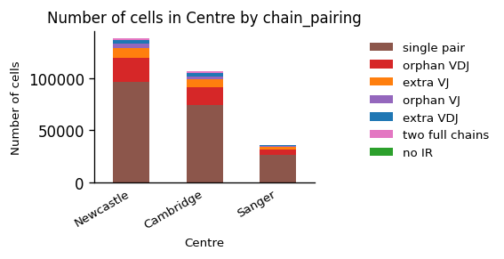
The data from all three centers contains mainly cells with a single pair of TCRs, which is a sign of good data quality. Often, we can compare different conditions better, when we view the fractions of cells in each condition instead of the absolute amount of cells:

_ = ir.pl.group_abundance(
    adata_tcr, groupby="Centre", target_col="chain_pairing", normalize=True
)

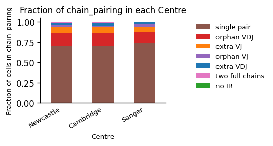
Here, we can see that all centers offer data of overall comparable data quality. The majority of T cells express a single TCR, followed by orphan VDJ, and VJ chains, which is typical when sequencing TCRs. Typical values of a good quality sample may be greater 60% single AIRs, 10-20% orphan chains, and ~10% extra chains. Note, that the percentage of cells without AIRs is naturally depending on the amount of non-AIR cells in the study, when sequencing multiple-modalities jointly.

_ = ir.pl.group_abundance(
    adata_tcr, groupby="Centre", target_col="receptor_type", normalize=True
)
_ = ir.pl.group_abundance(
    adata_tcr, groupby="Centre", target_col="receptor_subtype", normalize=True
)

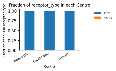
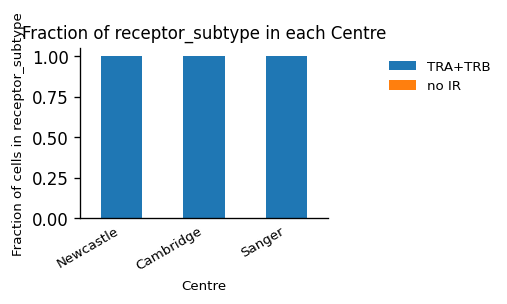
We can see, that the dataset consists only of TCRs (first plot), which is not surprising, since we have separated DataFrames of T - and B-cells. Additionally, the dataset only contains α/β-T cells. Since the amount of cells without IR cannot be recognized in the plot, we will look at the absolute numbers, and observe that only 22 cells have no AIR information. This fraction will be larger in most datasets, when sequencing multiple modalities depending on the amount of AIR cells.

adata_tcr.obs["chain_pairing"].value_counts()

single pair        196957
orphan VDJ          45266
extra VJ            19034
orphan VJ            7937
extra VDJ            7473
two full chains      3356
no IR                  22
Name: chain_pairing, dtype: int64

For the BCR, we will have a look at the patient-level. For visualization, we downsample to two patients (todo: later in line with rest downsampling):

adata_bcr_tmp = adata_bcr[
    adata_bcr.obs["patient_id"].isin(["COVID-003", "AP11"])
].copy()
_ = ir.pl.group_abundance(
    adata_bcr_tmp, groupby="patient_id", target_col="chain_pairing"
)
_ = ir.pl.group_abundance(
    adata_bcr_tmp, groupby="patient_id", target_col="chain_pairing", normalize=True
)

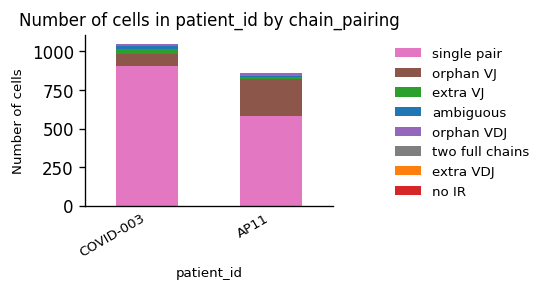
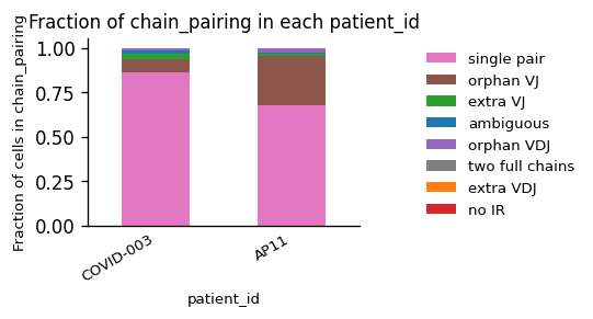
While we observe an considerable difference in the amount of B Cells between the patients, the quality of the chain pairings is comparable.

_ = ir.pl.group_abundance(
    adata_bcr_tmp, groupby="patient_id", target_col="receptor_type", normalize=True
)
_ = ir.pl.group_abundance(
    adata_bcr_tmp, groupby="patient_id", target_col="receptor_subtype", normalize=True
)

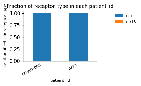
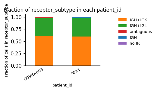
Again, we have only one type of AIR in the dataset (BCRs), but this time a mixture of κ- and λ-chains for the light chain.

38.9.3. Filtering

You might want to filter cells with different AIR states. Depending on your study, you have to decide the trade-off between the amount of data available and the quality of the data, when deciding for filtering. Often, all cells are kept within the dataset with their AIR state flagged. For different downstream analysis, only cells with correct information are then used. E.g. if you perform a database query based on CDR3-VDJ chain (see chapter X), it is possible to use orphan VDJ chains, while this is not possible when searching for the full AIR. In the following, we will show how the filtering is performed. It is up to the reader to decide, whether they want to perform the filtering at this point, or before the different analysis parts.

The filtering can be performed with various degrees of strictness and different combinations such as:

• has IR: keep only cells with expressed IRs, since we cannot perform sequence level analysis on them

• no multi chains: filter out cells with >2 AIRs to avoid doublets

• only one AIR: filter out cells with two AIRs or additional chains since specificity can not be attributed to a certain sequence

• no single chains: filter out cells with only VJ or VDJ chains, which cannot be used for all downstream analysis due to missing information

Since we will use the full data throughout this book, we will filter the data to a temporary AnnData object for each step described above. From the absolute cell numbers, you can see how many cells will be lost in each step.

adata_bcr_tmp.obs["chain_pairing"].value_counts()

single pair        1489
orphan VJ           312
extra VJ             46
ambiguous            31
orphan VDJ           25
two full chains       6
extra VDJ             4
no IR                 1
Name: chain_pairing, dtype: int64

print(f"Amount of all B cells:\t\t\t\t{len(adata_bcr)}")
adata_bcr_tmp = adata_bcr[adata_bcr.obs["chain_pairing"] != "no IR"]
print(f"Amount of B cells with AIR:\t\t\t{len(adata_bcr_tmp)}")

adata_bcr_tmp = adata_bcr_tmp[adata_bcr_tmp.obs["chain_pairing"] != "multi_chain"]
print(f"Amount of B cells without dublets:\t\t{len(adata_bcr_tmp)}")

adata_bcr_tmp = adata_bcr_tmp[
    ~adata_bcr_tmp.obs["chain_pairing"].isin(
        ["two full chains", "extra VJ", "extra VDJ"]
    )
]
print(f"Amount of B cells with unique AIR per cell:\t{len(adata_bcr_tmp)}")

adata_bcr_tmp = adata_bcr_tmp[adata_bcr_tmp.obs["chain_pairing"] == "single pair"]
print(f"Amount of B cells with sinlge complete AIR:\t{len(adata_bcr_tmp)}")

Amount of all B cells:				159446
Amount of B cells with AIR:			159185
Amount of B cells without dublets:		159185
Amount of B cells with unique AIR per cell:	153936
Amount of B cells with sinlge complete AIR:	108395

Eventually, we obtain an AnnData object with only single paired BCRs. However, the amount of data can be considerably smaller limiting downstream analysis.

adata_bcr_tmp.obs["chain_pairing"].value_counts()

single pair    108395
Name: chain_pairing, dtype: int64

Similarly, we can perform this filtering for the TCR data.

adata_tcr.obs["chain_pairing"].value_counts()

single pair        196957
orphan VDJ          45266
extra VJ            19034
orphan VJ            7937
extra VDJ            7473
two full chains      3356
no IR                  22
Name: chain_pairing, dtype: int64

print(f"Amount of all T cells:\t\t\t\t{len(adata_tcr)}")
adata_tcr_tmp = adata_tcr[adata_tcr.obs["chain_pairing"] != "no IR"]
print(f"Amount of T cells with AIR:\t\t\t{len(adata_tcr_tmp)}")

adata_tcr_tmp = adata_tcr_tmp[adata_tcr_tmp.obs["chain_pairing"] != "multi_chain"]
print(f"Amount of T cells without dublets:\t\t{len(adata_tcr_tmp)}")

adata_tcr_tmp = adata_tcr_tmp[
    ~adata_tcr_tmp.obs["chain_pairing"].isin(
        ["two full chains", "extra VJ", "extra VDJ"]
    )
]
print(f"Amount of T cells with unique AIR per cell:\t{len(adata_tcr_tmp)}")

adata_tcr_tmp = adata_tcr_tmp[adata_tcr_tmp.obs["chain_pairing"] == "single pair"]
print(f"Amount of T cells with sinlge complete AIR:\t{len(adata_tcr_tmp)}")

Amount of all T cells:				280045
Amount of T cells with AIR:			280023
Amount of T cells without dublets:		280023
Amount of T cells with unique AIR per cell:	250160
Amount of T cells with sinlge complete AIR:	196957

adata_tcr_tmp.obs["chain_pairing"].value_counts()

single pair    196957
Name: chain_pairing, dtype: int64

Finally, we save the annotated data for later analysis.

sc.write(adata=adata_tcr, filename=path_tcr_out)
sc.write(adata=adata_bcr, filename=path_bcr_out)

38.10. Key Takeaways

• VDJ-sequencing measures the sequence information of AIRs, which provides us insights into the function of B- and T-cells.

• To detect doublets, cells with multiple AIRs should be identified or filtered.

• Depending on the analysis, we additional filter cells with incomplete AIR information.

38.11. Quiz

Where does the high variability of AIRs stem from?

• + Junctional diversity adds random nucleotides.

• Peripheral diversity motivates rapid amino acid switches specific to the host organ.

• + Combinatorial diversity of different gene segments.

• Inherited diversity genetically encodes multiple AIRs.

What properties does a productive AIR have?

• + It spans over the V- to the J-gene with an CDR3 regions contained.

• It contains a stop codon in the D-gene.

• There exist multiple different sequences for the same AIR chains.

• + It contains a start codon in the leading region.

What cells should be identified for potential filtering?

• Cells with a high count of AIR sequence reads.

• + Cells with incomplete AIR information.

• + Cells with multiple AIRs indicating doublets.

• Cells with specific motifs in the CDR3 region.

38.12. References

[BBK20]

Nicholas Borcherding, Nicholas L Bormann, and Gloria Kraus. Screpertoire: an r-based toolkit for single-cell immune receptor analysis. F1000Research, 2020.

[BIJB19]

Bryan Briney, Anne Inderbitzin, Collin Joyce, and Dennis R Burton. Commonality despite exceptional diversity in the baseline human antibody repertoire. Nature, 566(7744):393–397, 2019.

[CNT+16]

Stefan Canzar, Karlynn E Neu, Qingming Tang, Patrick C Wilson, and Aly A Khan. BASIC: BCR assembly from single cells. Bioinformatics, 33(3):425–427, 10 2016. URL: https://doi.org/10.1093/bioinformatics/btw631, arXiv:https://academic.oup.com/bioinformatics/article-pdf/33/3/425/25145999/btw631.pdf, doi:10.1093/bioinformatics/btw631.

[CA06]

Max D Cooper and Matthew N Alder. The evolution of adaptive immune systems. Cell, 124(4):815–822, 2006.

[HZXD16]

Ping Hu, Wenhua Zhang, Hongbo Xin, and Glenn Deng. Single cell isolation and analysis. Frontiers in cell and developmental biology, 4:116, 2016.

[LEM+18]

Ida Lindeman, Guy Emerton, Lira Mamanova, Omri Snir, Krzysztof Polanski, Shuo-Wang Qiao, Ludvig M. Sollid, Sarah A. Teichmann, and Michael J. T. Stubbington. Bracer: b-cell-receptor reconstruction and clonality inference from single-cell rna-seq. Nature Methods, 15(8):563–565, Aug 2018. URL: https://doi.org/10.1038/s41592-018-0082-3, doi:10.1038/s41592-018-0082-3.

[SB19] (1,2)

Nathaniel J Schuldt and Bryce A Binstadt. Dual tcr t cells: identity crisis or multitaskers? The Journal of Immunology, 202(3):637–644, 2019.

[SAEC+19]

Mandeep Singh, Ghamdan Al-Eryani, Shaun Carswell, James M Ferguson, James Blackburn, Kirston Barton, Daniel Roden, Fabio Luciani, Tri Giang Phan, Simon Junankar, and others. High-throughput targeted long-read single cell sequencing reveals the clonal and transcriptional landscape of lymphocytes. Nature communications, 10(1):1–13, 2019.

[SRB+21] (1,2)

Emily Stephenson, Gary Reynolds, Rachel A Botting, Fernando J Calero-Nieto, Michael D Morgan, Zewen Kelvin Tuong, Karsten Bach, Waradon Sungnak, Kaylee B Worlock, Masahiro Yoshida, and others. Single-cell multi-omics analysis of the immune response in covid-19. Nature medicine, 27(5):904–916, 2021.

[SSF+20]

Gregor Sturm, Tamas Szabo, Georgios Fotakis, Marlene Haider, Dietmar Rieder, Zlatko Trajanoski, and Francesca Finotello. Scirpy: a scanpy extension for analyzing single-cell t-cell receptor-sequencing data. Bioinformatics, 36(18):4817–4818, 2020.

[UKW+18]

Amit A. Upadhyay, Robert C. Kauffman, Amber N. Wolabaugh, Alice Cho, Nirav B. Patel, Samantha M. Reiss, Colin Havenar-Daughton, Reem A. Dawoud, Gregory K. Tharp, Iñaki Sanz, Bali Pulendran, Shane Crotty, F. Eun-Hyung Lee, Jens Wrammert, and Steven E. Bosinger. Baldr: a computational pipeline for paired heavy and light chain immunoglobulin reconstruction in single-cell rna-seq data. Genome Medicine, 10(1):20, Mar 2018. URL: https://doi.org/10.1186/s13073-018-0528-3, doi:10.1186/s13073-018-0528-3.

[VdVG+22]

Sebastiaan Valkiers, Nicky de Vrij, Sofie Gielis, Sara Verbandt, Benson Ogunjimi, Kris Laukens, and Pieter Meysman. Recent advances in t-cell receptor repertoire analysis: bridging the gap with multimodal single-cell rna sequencing. ImmunoInformatics, pages 100009, 2022.

[WAT18]

F Alexander Wolf, Philipp Angerer, and Fabian J Theis. Scanpy: large-scale single-cell gene expression data analysis. Genome biology, 19(1):1–5, 2018.

[YAK+21]

Alexander Yermanos, Andreas Agrafiotis, Raphael Kuhn, Damiano Robbiani, Josephine Yates, Chrysa Papadopoulou, Jiami Han, Ioana Sandu, Cédric Weber, Florian Bieberich, and others. Platypus: an open-access software for integrating lymphocyte single-cell immune repertoires with transcriptomes. NAR genomics and bioinformatics, 3(2):lqab023, 2021.

[ZES+13]

Veronika Zarnitsyna, Brian Evavold, Louie Schoettle, Joseph Blattman, and Rustom Antia. Estimating the diversity, completeness, and cross-reactivity of the t cell repertoire. Frontiers in immunology, 4:485, 2013.

[ImmunoMindTeam19]

ImmunoMind Team. immunarch: An R Package for Painless Bioinformatics Analysis of T-Cell and B-Cell Immune Repertoires. August 2019. URL: https://doi.org/10.5281/zenodo.3367200, doi:10.5281/zenodo.3367200.