44. Paired integration#
Key takeaways
The integration of single-cell multi-modal data (e.g., gene expression and chromatin accessibility) is challenging due to differences in dimensionality and data distributions across modalities, but tools like MOFA+, WNN, totalVI, and multiVI aim to address these challenges.
Query-to-reference mapping allows for the integration of new data into a pre-existing reference framework, enabling tasks like cell type prediction and imputation of missing modalities (e.g., predicting protein abundance from RNA-seq data)
Environment setup
Install conda:
Before creating the environment, ensure that conda is installed on your system.
Save the yml content:
Copy the content from the yml tab into a file named
environment.yml.
Create the environment:
Open a terminal or command prompt.
Run the following command:
conda env create -f environment.yml
Activate the environment:
After the environment is created, activate it using:
conda activate <environment_name>
Replace
<environment_name>with the name specified in theenvironment.ymlfile. In the yml file it will look like this:name: <environment_name>
Verify the installation:
Check that the environment was created successfully by running:
conda env list
name: paired-integration
channels:
  - conda-forge
  - bioconda
  - defaults
dependencies:
  - conda-forge::python=3.12
  - conda-forge::scanpy=1.11.5
  - conda-forge::r-base=4.4
  - conda-forge::r-seurat=5.1
  - bioconda::bioconductor-singlecellexperiment
  - conda-forge::rpy2=3.6
  - bioconda::anndata2ri=1.3
  - conda-forge::pytorch-cpu
  - conda-forge::pip
  - pip:
      - muon==0.1.7
      - pysam
      - mofapy2==0.7.2
      - scib==1.1.6
      - scvi-tools==1.4.1
44.1. Motivation#
In the recent years several technologies appeared that allow us to measure several modalities in a single-cell. Modalities in this context refer to different type of information that we can capture in each cell. For instance, CITE-seq allows measuring gene expression and surface protein abundance in the same cell. Alternatively, paired RNA-seq/ATAC-seq experiments using, for example, the Multiome assay, capture gene expression and chromatin accessibility simultaneously.
We are interested in the most holistic representation of single cells that incorporate information from all the available modalities, but several challenges might arise when integrating these different modalities. Data stemming from different sequencing technologies can vary in dimensions: RNA-seq experiments usually capture 20-30 thousand genes, but the protein panel can be as small just a few proteins up to 200. ATAC-seq experiments on the other hand can have more than 200000 peaks. On top of having different dimensionality, the data can follow different distributions. RNA-seq counts are often modelled with negative binomial distribution, while chromatin accessibility can be binarized and modelled as either open or closed and therefore with a Bernoulli distribution [Ashuach et al., 2021]. Alternatively raw ATAC-seq counts can be modelled following Poisson distribution [Martens et al., 2022].
Here, we showcase several tools for paired integration including MOFA+ [Argelaguet et al., 2020], WNN [Hao et al., 2021], totalVI [Gayoso et al., 2021] and multiVI [Ashuach et al., 2021]. We use 10x Multiome and CITE-seq data generated for the single cell data integration challenge at the NeurIPS conference 2021 [Luecken et al., 2021]. This dataset captures single-cell data from bone marrow mononuclear cells of 12 healthy human donors measured at four different sites to obtain nested batch effects. In this tutorial, we will use 3 batches from one site to showcase the integration tools.
Since there are multiple integration tools available, it can be quite challenging to assess which tool to use for a particular task at hand. We therefore use the scIB [Luecken et al., 2022] package that allows to make such a decision by quantitatively assessing the quality of the integration. It is important to note though that scIB was designed for unimodal integration of batches and not for multimodal integration. We expect more metrics to appear in the near future that are specifically designed for multimodal data, but for now we show how to use scIB metrics to compare the integration results.
44.2. Environment setup#
import logging

import anndata as ad
import anndata2ri
import matplotlib.pyplot as plt
import muon as mu
import pandas as pd
import rpy2.rinterface_lib.callbacks
import scanpy as sc
import scib
import scipy
import scipy.io
import scvi
import seaborn as sns
from rpy2.robjects import pandas2ri

rpy2.rinterface_lib.callbacks.logger.setLevel(logging.ERROR)

pandas2ri.activate()
anndata2ri.activate()

%load_ext rpy2.ipython

import warnings

warnings.filterwarnings("ignore")
During startup - Warning message:
Setting LC_CTYPE failed, using "C"
Global seed set to 0
/lustre/groups/ml01/workspace/anastasia.litinetskaya/miniconda3/envs/paired_integration_chapter/lib/python3.9/site-packages/pytorch_lightning/utilities/warnings.py:53: LightningDeprecationWarning: pytorch_lightning.utilities.warnings.rank_zero_deprecation has been deprecated in v1.6 and will be removed in v1.8. Use the equivalent function from the pytorch_lightning.utilities.rank_zero module instead.
  new_rank_zero_deprecation(
/lustre/groups/ml01/workspace/anastasia.litinetskaya/miniconda3/envs/paired_integration_chapter/lib/python3.9/site-packages/pytorch_lightning/utilities/warnings.py:58: LightningDeprecationWarning: The `pytorch_lightning.loggers.base.rank_zero_experiment` is deprecated in v1.7 and will be removed in v1.9. Please use `pytorch_lightning.loggers.logger.rank_zero_experiment` instead.
  return new_rank_zero_deprecation(*args, **kwargs)
/lustre/groups/ml01/workspace/anastasia.litinetskaya/miniconda3/envs/paired_integration_chapter/lib/python3.9/site-packages/rpy2/robjects/pandas2ri.py:351: DeprecationWarning: The global conversion available with activate() is deprecated and will be removed in the next major release. Use a local converter.
  warnings.warn('The global conversion available with activate() '
/lustre/groups/ml01/workspace/anastasia.litinetskaya/miniconda3/envs/paired_integration_chapter/lib/python3.9/site-packages/rpy2/robjects/numpy2ri.py:226: DeprecationWarning: The global conversion available with activate() is deprecated and will be removed in the next major release. Use a local converter.
  warnings.warn('The global conversion available with activate() '
/lustre/groups/ml01/workspace/anastasia.litinetskaya/miniconda3/envs/paired_integration_chapter/lib/python3.9/site-packages/rpy2/robjects/conversion.py:28: DeprecationWarning: The use of converter in module rpy2.robjects.conversion is deprecated. Use rpy2.robjects.conversion.get_conversion() instead of rpy2.robjects.conversion.converter.
  warnings.warn(
%%R
suppressPackageStartupMessages({
    library(Seurat)
})
set.seed(123)
    WARNING: The R package "reticulate" only fixed recently
    an issue that caused a segfault when used with rpy2:
    https://github.com/rstudio/reticulate/pull/1188
    Make sure that you use a version of that package that includes
    the fix.
44.3. CITE-seq data#
We first show how to integrate a CITE-seq dataset using WNN, MOFA+ and totalVI. CITE-seq data contains raw gene expression counts and counts for surface proteins. The surface protein data is represented as antibody-derived tags (adt) here. We refer to the Quality control section of the Surface Proteins chapter for more details.
44.3.1. Prepare data#
adt = sc.read(
    "/lustre/groups/ml01/workspace/anastasia.litinetskaya/data/neurips-cite/adt_pp.h5ad"
)
adt
AnnData object with n_obs × n_vars = 120502 × 136
    obs: 'donor', 'batch', 'n_genes_by_counts', 'log1p_n_genes_by_counts', 'total_counts', 'log1p_total_counts', 'n_counts', 'outliers'
    var: 'gene_ids', 'feature_types', 'n_cells_by_counts', 'mean_counts', 'log1p_mean_counts', 'pct_dropout_by_counts', 'total_counts', 'log1p_total_counts'
    uns: 'batch_colors', 'donor_colors', 'neighbors', 'pca', 'umap'
    obsm: 'X_isotypes', 'X_pca', 'X_pcahm', 'X_umap'
    varm: 'PCs'
    layers: 'counts'
    obsp: 'connectivities', 'distances'
rna = sc.read(
    "/lustre/groups/ml01/workspace/anastasia.litinetskaya/data/neurips-cite/rna_hvg.h5ad"
)
rna
AnnData object with n_obs × n_vars = 90261 × 4000
    obs: 'GEX_n_genes_by_counts', 'GEX_pct_counts_mt', 'GEX_size_factors', 'GEX_phase', 'ADT_n_antibodies_by_counts', 'ADT_total_counts', 'ADT_iso_count', 'cell_type', 'batch', 'ADT_pseudotime_order', 'GEX_pseudotime_order', 'Samplename', 'Site', 'DonorNumber', 'Modality', 'VendorLot', 'DonorID', 'DonorAge', 'DonorBMI', 'DonorBloodType', 'DonorRace', 'Ethnicity', 'DonorGender', 'QCMeds', 'DonorSmoker', 'is_train'
    var: 'feature_types', 'gene_id', 'highly_variable', 'means', 'dispersions', 'dispersions_norm'
    uns: 'dataset_id', 'genome', 'hvg', 'organism'
    obsm: 'ADT_X_pca', 'ADT_X_umap', 'ADT_isotype_controls', 'GEX_X_pca', 'GEX_X_umap'
    layers: 'counts'
We subset the data to Site 1 and the 3 corresponding donors to reduce the run time.
batches_to_keep = ["s1d1", "s1d2", "s1d3"]
rna = rna[rna.obs["batch"].isin(batches_to_keep)]
adt = adt[adt.obs["donor"].isin(batches_to_keep)]
We only keep the cells that are present in both modality objects. First we need to make sure that .obs_names of both objects have similar structure and if not clean up a bit.
adt.obs_names
Index(['AAACCCAAGGATGGCT-1-0-0-0-0-0-0-0-0-0-0-0',
       'AAACCCAAGGCCTAGA-1-0-0-0-0-0-0-0-0-0-0-0',
       'AAACCCAAGTGAGTGC-1-0-0-0-0-0-0-0-0-0-0-0',
       'AAACCCACAAGAGGCT-1-0-0-0-0-0-0-0-0-0-0-0',
       'AAACCCACATCGTGGC-1-0-0-0-0-0-0-0-0-0-0-0',
       'AAACCCACATTCTCTA-1-0-0-0-0-0-0-0-0-0-0-0',
       'AAACCCAGTCCGCAGT-1-0-0-0-0-0-0-0-0-0-0-0',
       'AAACCCAGTGCATACT-1-0-0-0-0-0-0-0-0-0-0-0',
       'AAACCCAGTTGACGGA-1-0-0-0-0-0-0-0-0-0-0-0',
       'AAACCCATCGATACTG-1-0-0-0-0-0-0-0-0-0-0-0',
       ...
       'TTTGGTTCATGTTACG-1-1-0-0-0', 'TTTGGTTGTCTCACAA-1-1-0-0-0',
       'TTTGGTTTCCCATTCG-1-1-0-0-0', 'TTTGGTTTCCGTCCTA-1-1-0-0-0',
       'TTTGGTTTCTTGCGCT-1-1-0-0-0', 'TTTGTTGAGAGTCTGG-1-1-0-0-0',
       'TTTGTTGCAGACAATA-1-1-0-0-0', 'TTTGTTGCATGTTACG-1-1-0-0-0',
       'TTTGTTGGTAGTCACT-1-1-0-0-0', 'TTTGTTGTCGCGCTGA-1-1-0-0-0'],
      dtype='object', length=24326)
rna.obs_names
Index(['GCATTAGCATAAGCGG-1-s1d1', 'TACAGGTGTTAGAGTA-1-s1d1',
       'AGGATCTAGGTCTACT-1-s1d1', 'GTAGAAAGTGACACAG-1-s1d1',
       'TCCGAAAAGGATCATA-1-s1d1', 'CTCCCAATCCATTGGA-1-s1d1',
       'GACCAATCAATTTCGG-1-s1d1', 'TTCCGGTAGTTGTAAG-1-s1d1',
       'ACCTGTCAGGACTGGT-1-s1d1', 'TTCGATTTCAGGACAG-1-s1d1',
       ...
       'GTGGTTAGTCGAGTTT-1-s1d3', 'TGAGACTCAATAGTAG-1-s1d3',
       'CATGAGTTCAGCAGAG-1-s1d3', 'GCTACAACAGTGCGCT-1-s1d3',
       'AGAAATGAGTGCCTCG-1-s1d3', 'AACAAAGGTTGGTACT-1-s1d3',
       'TGACAGTCATGGCTGC-1-s1d3', 'CTGGCAGGTCTCACGG-1-s1d3',
       'GTAACCATCGGAGTGA-1-s1d3', 'GAGTTGTCAGTCGGAA-1-s1d3'],
      dtype='object', length=16311)
adt.obs_names = [
    name.split("-")[0] + "-" + name.split("-")[1] + "-" + batch
    for batch, name in zip(adt.obs["donor"], adt.obs_names, strict=False)
]
common_idx = list(set(rna.obs_names).intersection(set(adt.obs_names)))
rna = rna[common_idx].copy()
adt = adt[common_idx].copy()
We need to rename the proteins in the adt object so that the gene names and protein names do not intersect.
adt.var_names = ["PROT_" + name for name in adt.var_names]
Next we create a MuData object where we store data for both modalities.
mdata = mu.MuData({"rna": rna, "adt": adt})
mdata
MuData object with n_obs × n_vars = 16294 × 4136
  var:	'feature_types'
  2 modalities
    rna:	16294 x 4000
      obs:	'GEX_n_genes_by_counts', 'GEX_pct_counts_mt', 'GEX_size_factors', 'GEX_phase', 'ADT_n_antibodies_by_counts', 'ADT_total_counts', 'ADT_iso_count', 'cell_type', 'batch', 'ADT_pseudotime_order', 'GEX_pseudotime_order', 'Samplename', 'Site', 'DonorNumber', 'Modality', 'VendorLot', 'DonorID', 'DonorAge', 'DonorBMI', 'DonorBloodType', 'DonorRace', 'Ethnicity', 'DonorGender', 'QCMeds', 'DonorSmoker', 'is_train'
      var:	'feature_types', 'gene_id', 'highly_variable', 'means', 'dispersions', 'dispersions_norm'
      uns:	'dataset_id', 'genome', 'hvg', 'organism'
      obsm:	'ADT_X_pca', 'ADT_X_umap', 'ADT_isotype_controls', 'GEX_X_pca', 'GEX_X_umap'
      layers:	'counts'
    adt:	16294 x 136
      obs:	'donor', 'batch', 'n_genes_by_counts', 'log1p_n_genes_by_counts', 'total_counts', 'log1p_total_counts', 'n_counts', 'outliers'
      var:	'gene_ids', 'feature_types', 'n_cells_by_counts', 'mean_counts', 'log1p_mean_counts', 'pct_dropout_by_counts', 'total_counts', 'log1p_total_counts'
      uns:	'batch_colors', 'donor_colors', 'neighbors', 'pca', 'umap'
      obsm:	'X_isotypes', 'X_pca', 'X_pcahm', 'X_umap'
      varm:	'PCs'
      layers:	'counts'
      obsp:	'connectivities', 'distances'
We copy batch and cell_type column from one of the modality adatas to .obs of the mdata object to later use for visualizations.
mdata.obs["batch"] = rna.obs["batch"].copy()
mdata.obs["cell_type"] = rna.obs["cell_type"].copy()
44.3.2. Weighted Nearest Neighbor (WNN)#
WNN is a graph-based method that takes neighbor graphs for each modality and constructs a common graph which is a weighted combination of the modality graphs. This constructed WNN graph can later be used together with gene expression matrix to obtain a supervised PCA (sPCA) representation guided by a WNN graph. The sPCA representation can be viewed as an embedding in a latent space.
First, we use the anndata2ri package (theislab/anndata2ri) to move Python AnnData object to SingleCellExperiment and Seurat R objects. We create slimmer versions of AnnData objects that only contain the information that we need for the analysis.
adata_ = ad.AnnData(adt.X.copy())
adata_.obs_names = adt.obs_names.copy()
adata_.var_names = adt.var_names.copy()
adata_.obs["batch"] = adt.obs["donor"].copy()
adata_.obsm["harmony_pca"] = adt.obsm["X_pcahm"].copy()
%%R -i adata_
# indicate that data is stored in .X of AnnData object
adt = as.Seurat(adata_, data='X', counts=NULL)
# the assay is called "originalexp" by default, we rename it to "ADT"
adt <- RenameAssays(object = adt, originalexp = "ADT", verbose=FALSE)
adt
An object of class Seurat
136 features across 16294 samples within 1 assay
Active assay: ADT (136 features, 0 variable features)
 1 dimensional reduction calculated: harmony_pca
We repeat the same for RNA data.
adata_ = ad.AnnData(rna.X.copy())
adata_.obs_names = rna.obs_names.copy()
adata_.var_names = rna.var_names.copy()
adata_.obs["cell_type"] = rna.obs["cell_type"].copy()
adata_.obs["batch"] = rna.obs["batch"].copy()
%%R -i adata_
rna = as.Seurat(adata_, data='X', counts=NULL)
rna
An object of class Seurat
4000 features across 16294 samples within 1 assay
Active assay: originalexp (4000 features, 0 variable features)
Next we create a Seurat object with both assays.
%%R
cite <- rna
cite[["ADT"]] <- CreateAssayObject(data = adt@assays$ADT@data)
%%R
cite <- RenameAssays(object = cite, originalexp = "RNA", verbose=FALSE)
Since we have several batches in the dataset, we would need to perform batch correction before integrating the modalities. One option would be to batch correct using Seurat’s FindIntegrationAnchors() and IntegrateData() (see https://satijalab.org/seurat/articles/integration_introduction.html) functions separately for each modality. We will use batch corrected embedding from previous analysis done separately for ADT and RNA data, namely Harmony corrected PCA embedding for ADT and scVI batch-corrected latent embedding for RNA.
%%R
# TODO need to change after we have the preprocessed data, for now RNA is not batch-corrected
DefaultAssay(cite) <- "RNA"
VariableFeatures(cite) <- rownames(cite)
cite <- ScaleData(cite, verbose=FALSE)
cite <- RunPCA(cite, verbose=FALSE)
%%R
cite@reductions$harmony_pca <- adt@reductions$harmony_pca
cite
An object of class Seurat
4136 features across 16294 samples within 2 assays
Active assay: RNA (4000 features, 4000 variable features)
 1 other assay present: ADT
 2 dimensional reductions calculated: pca, harmony_pca
Now we follow the WNN vignette to perform the analysis. First, we need to find multimodal neighbors using the specified dimensionality reductions for each of the modalities. This function adds a WNN graph to the Seurat object.
%%R
cite <- FindMultiModalNeighbors(
    cite,
    reduction.list = list("pca", "harmony_pca"),
    dims.list = list(1:50, 1:30),
    modality.weight.name = "RNA.weight",
    verbose = FALSE
)
Since we are also interested in finding an embedding for our multimodal data, we additionally run the RunSPCA() function that uses RNA gene expression data and the WNN graph for supervised PCA. Supervised PCA is a “guided” version of standard PCA run on gene expression data guided by the WNN graph to better preserve relationships between cells learned in WNN graph. We also will need a reference UMAP later for mapping an RNA query onto this multimodal reference as discussed in Advanced integration.
%%R
cite <- RunSPCA(cite, assay = "RNA", graph = "wsnn", npcs = 20)
cite <- RunUMAP(cite, nn.name = "weighted.nn", reduction.name = "wnn.umap", reduction.key = "wnnUMAP_", return.model=TRUE)
%%R
cite
An object of class Seurat
4136 features across 16294 samples within 2 assays
Active assay: RNA (4000 features, 4000 variable features)
 1 other assay present: ADT
 4 dimensional reductions calculated: pca, harmony_pca, spca, wnn.umap
We save the Seurat object as an .rds file for the Advanced integration section.
%%R
saveRDS(cite, file = "wnn_ref.rds")
We move the sPCA embedding to Python and store them in .obsm of the MuData object.
%%R -o spca
spca = Embeddings(object = cite[["spca"]])
mdata.obsm["X_spca"] = spca
We also need to extract the calculated WNN graph.
%%R -o wnn
wnn <- as.data.frame(summary(cite@graphs$wknn))
The table indicates indices with connections between cells in the WNN graph. Since R starts indexing at 1 but Python at 0, we modify the indices to start with 0.
wnn[:5]
| i | j | x | |
|---|---|---|---|
| 1 | 1 | 1 | 1.0 |
| 2 | 202 | 1 | 1.0 |
| 3 | 787 | 1 | 1.0 |
| 4 | 1628 | 1 | 1.0 |
| 5 | 2076 | 1 | 1.0 |
wnn["i"] = wnn["i"] - 1
wnn["j"] = wnn["j"] - 1
wnn[:5]
| i | j | x | |
|---|---|---|---|
| 1 | 0 | 0 | 1.0 |
| 2 | 201 | 0 | 1.0 |
| 3 | 786 | 0 | 1.0 |
| 4 | 1627 | 0 | 1.0 |
| 5 | 2075 | 0 | 1.0 |
We store the graph in .obsp of the MuData object.
mdata.obsp["wnn_connectivities"] = scipy.sparse.coo_matrix(
    (wnn["x"], (wnn["i"], wnn["j"]))
)
Next we use the WNN graph to calculate the UMAP coordinates and save them in .obsm['X_umap_wnn']. We could alternatively also just use sPCA coordinates for visualization.
# we won't actually need the neighbors
# but need to run this anyway as a little trick to make scanpy work with externally-computed neighbors
sc.pp.neighbors(mdata, use_rep="X_spca")
mdata.obsp["connectivities"] = mdata.obsp["wnn_connectivities"].copy()
# delete distances to make sure we are not using anything calculated with sc.pp.neighbors()
del mdata.obsp["distances"]
sc.tl.umap(mdata)
mdata.obsm["X_umap_wnn"] = mdata.obsm["X_umap"].copy()
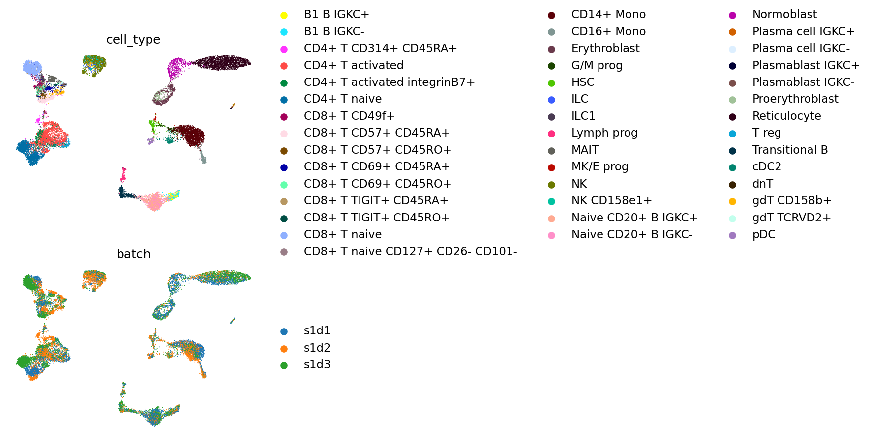
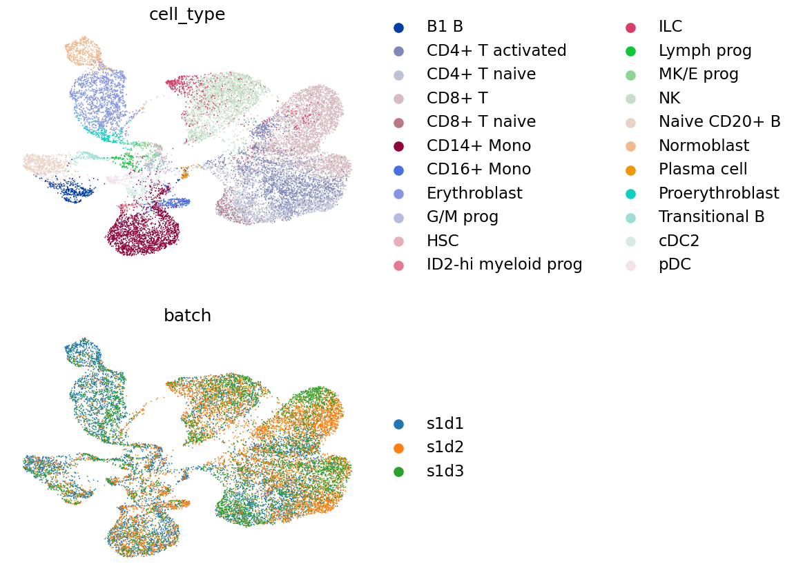
Finally we visualize the cell types and batches on a UMAP.
mu.pl.embedding(
    mdata, color=["cell_type", "batch"], ncols=1, basis="umap_wnn", frameon=False
)
To be able to quantitatively assess the result of the integration and compare to other methods we compute some of the scIB metrics using the sPCA embedding and WNN graph. More specifically, we calculate the following metrics:
bio conservation:
NMI_cluster/label,ARI_cluster/label,ASW_labelandisolated_label_silhouette;batch correction:
ASW_label/batch,graph_conn.
scib_anndata = sc.AnnData(mdata.obsm["X_spca"]).copy()
scib_anndata.obs = mdata.obs.copy()
scib_anndata.obsp["connectivities"] = mdata.obsp["connectivities"].copy()
scib_anndata.obsm["X_spca"] = mdata.obsm["X_spca"].copy()
metrics_wnn = scib.metrics.metrics(
    scib_anndata,
    scib_anndata,
    batch_key="batch",
    label_key="cell_type",
    embed="X_spca",
    ari_=True,
    nmi_=True,
    silhouette_=True,
    graph_conn_=True,
    isolated_labels_asw_=True,
)
metrics_wnn
NMI...
ARI...
Silhouette score...
Isolated labels ASW...
Graph connectivity...
| 0 | |
|---|---|
| NMI_cluster/label | 0.808672 |
| ARI_cluster/label | 0.729036 |
| ASW_label | 0.595822 |
| ASW_label/batch | 0.854867 |
| PCR_batch | NaN |
| cell_cycle_conservation | NaN |
| isolated_label_F1 | NaN |
| isolated_label_silhouette | 0.420527 |
| graph_conn | 0.914140 |
| kBET | NaN |
| iLISI | NaN |
| cLISI | NaN |
| hvg_overlap | NaN |
| trajectory | NaN |
We note that even though batch correction was performed using Harmony for ADT and scVI for RNA, we still include metrics that assess batch correction here too.
44.3.3. Multi-Omics Factor Analysis (MOFA+)#
MOFA+ is a linear factor model that decomposes the input matrices into the product of low-rank matrices. The low-rank representation can be used as an embedding in a low-dimensional space for visualization and other downstream tasks. The latent dimensions are interpretable with respect to the original input features and represent the leading sources of variation in the data.
By default, we are using data from .X and the data should be normalized. Since there are some batch effects in the data that MOFA+ can correct for, we also pass the groups_label parameter to specify the batch covariate.
If you want to run MOFA+ on a GPU, you need to additionally install a version of cuPY (https://cupy.dev) which is compatible with your CUDA.
mu.tl.mofa(mdata, groups_label="batch", gpu_mode=True)
        #########################################################
        ###           __  __  ____  ______                    ###
        ###          |  \/  |/ __ \|  ____/\    _             ###
        ###          | \  / | |  | | |__ /  \ _| |_           ###
        ###          | |\/| | |  | |  __/ /\ \_   _|          ###
        ###          | |  | | |__| | | / ____ \|_|            ###
        ###          |_|  |_|\____/|_|/_/    \_\              ###
        ###                                                   ###
        #########################################################


Loaded view='rna' group='s1d1' with N=5219 samples and D=4000 features...
Loaded view='rna' group='s1d3' with N=4975 samples and D=4000 features...
Loaded view='rna' group='s1d2' with N=6100 samples and D=4000 features...
Loaded view='adt' group='s1d1' with N=5219 samples and D=136 features...
Loaded view='adt' group='s1d3' with N=4975 samples and D=136 features...
Loaded view='adt' group='s1d2' with N=6100 samples and D=136 features...


Model options:
- Automatic Relevance Determination prior on the factors: True
- Automatic Relevance Determination prior on the weights: True
- Spike-and-slab prior on the factors: False
- Spike-and-slab prior on the weights: True
Likelihoods:
- View 0 (rna): gaussian
- View 1 (adt): gaussian


GPU mode is activated


######################################
## Training the model with seed 1 ##
######################################


Converged!


#######################
## Training finished ##
#######################


Saving model in /tmp/mofa_20230103-162506.hdf5...
Saved MOFA embeddings in .obsm['X_mofa'] slot and their loadings in .varm['LFs'].
We use the X_mofa representation to calculate the neighbors and the UMAP coordinates, and store them in .obsm['X_umap_mofa'].
sc.pp.neighbors(mdata, use_rep="X_mofa")
sc.tl.umap(mdata)
mdata.obsm["X_umap_mofa"] = mdata.obsm["X_umap"].copy()
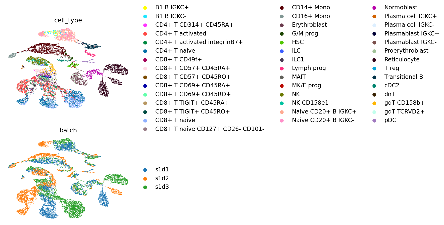
We plot the cell types and batches again on the resulting UMAP.
mu.pl.embedding(
    mdata, color=["cell_type", "batch"], ncols=1, basis="umap_mofa", frameon=False
)
Finally, we calculate the same scIB metrics as before.
scib_anndata = sc.AnnData(mdata.obsm["X_mofa"]).copy()
scib_anndata.obs = mdata.obs.copy()
scib_anndata.obsp["connectivities"] = mdata.obsp["connectivities"].copy()
scib_anndata.obsm["X_mofa"] = mdata.obsm["X_mofa"].copy()
metrics_mofa = scib.metrics.metrics(
    scib_anndata,
    scib_anndata,
    batch_key="batch",
    label_key="cell_type",
    embed="X_mofa",
    ari_=True,
    nmi_=True,
    silhouette_=True,
    graph_conn_=True,
    isolated_labels_asw_=True,
)
metrics_mofa
NMI...
ARI...
Silhouette score...
Isolated labels ASW...
Graph connectivity...
| 0 | |
|---|---|
| NMI_cluster/label | 0.727261 |
| ARI_cluster/label | 0.497166 |
| ASW_label | 0.566888 |
| ASW_label/batch | 0.800875 |
| PCR_batch | NaN |
| cell_cycle_conservation | NaN |
| isolated_label_F1 | NaN |
| isolated_label_silhouette | 0.418293 |
| graph_conn | 0.886662 |
| kBET | NaN |
| iLISI | NaN |
| cLISI | NaN |
| hvg_overlap | NaN |
| trajectory | NaN |
44.3.4. Total Variational Inference (totalVI)#
TotalVI is a variational-inference-based method for joint analysis of paired gene expression and protein abundance measurements. It takes into account batch effects, protein background noise, which allows the model to learn a joint latent representation disentangled from technical factors. TotalVI models transcriptome counts with negative-binomial (NB) distribution and the protein counts as NB mixture of foreground and background signal. Hence, the model takes raw gene expression and raw protein counts as input.
adata = mdata["rna"].copy()
adata.obsm["protein_expression"] = mdata["adt"].layers["counts"].A.copy()
We need to specify that raw counts for RNA are stored in counts layer of our adata and that we want to correct for batch effect with batch_key="batch" parameter.
scvi.model.TOTALVI.setup_anndata(
    adata,
    protein_expression_obsm_key="protein_expression",
    layer="counts",
    batch_key="batch",
)
No GPU/TPU found, falling back to CPU. (Set TF_CPP_MIN_LOG_LEVEL=0 and rerun for more info.)
INFO Generating sequential column names
We initialize the totalVI model.
vae = scvi.model.TOTALVI(adata)
INFO Computing empirical prior initialization for protein background.
Next, we train the model with default parameters.
vae.train()
GPU available: True (cuda), used: True
TPU available: False, using: 0 TPU cores
IPU available: False, using: 0 IPUs
HPU available: False, using: 0 HPUs
LOCAL_RANK: 0 - CUDA_VISIBLE_DEVICES: [0]
Epoch 340/400:  85%|████████▌ | 340/400 [08:00<01:22,  1.37s/it, loss=1.65e+03, v_num=1]Epoch 00340: reducing learning rate of group 0 to 2.4000e-03.
Epoch 400/400: 100%|██████████| 400/400 [09:22<00:00,  1.37s/it, loss=1.64e+03, v_num=1]
`Trainer.fit` stopped: `max_epochs=400` reached.
Epoch 400/400: 100%|██████████| 400/400 [09:22<00:00, 1.41s/it, loss=1.64e+03, v_num=1]
Next, we obtain the latent representation and store it in .obsm['X_totalVI'] and then use it to calculate the UMAP coordinates.
mdata.obsm["X_totalVI"] = vae.get_latent_representation()
sc.pp.neighbors(mdata, use_rep="X_totalVI")
sc.tl.umap(mdata)
mdata.obsm["X_umap_totalVI"] = mdata.obsm["X_umap"].copy()
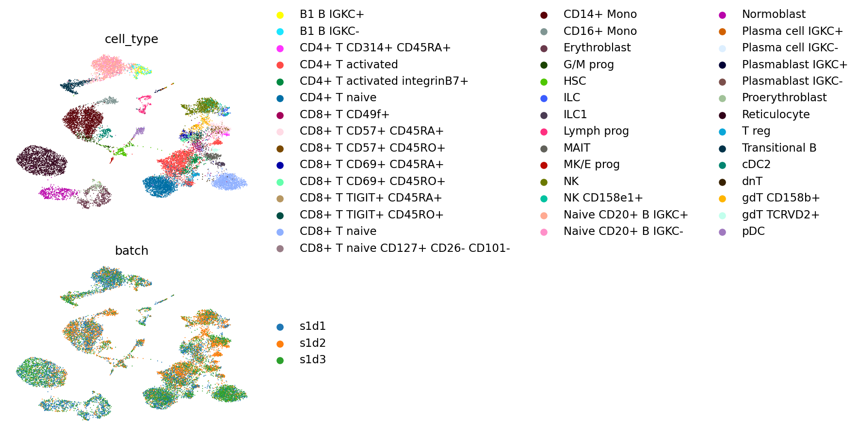
As above, we plot cell types and batches on a UMAP.
mu.pl.embedding(
    mdata, color=["cell_type", "batch"], ncols=1, basis="umap_totalVI", frameon=False
)
And finally, we calculate scIB metrics.
scib_anndata = sc.AnnData(mdata.obsm["X_totalVI"]).copy()
scib_anndata.obs = mdata.obs.copy()
scib_anndata.obsp["connectivities"] = mdata.obsp["connectivities"].copy()
scib_anndata.obsm["X_totalVI"] = mdata.obsm["X_totalVI"].copy()
metrics_totalvi = scib.metrics.metrics(
    scib_anndata,
    scib_anndata,
    batch_key="batch",
    label_key="cell_type",
    embed="X_totalVI",
    ari_=True,
    nmi_=True,
    silhouette_=True,
    graph_conn_=True,
    isolated_labels_asw_=True,
)
metrics_totalvi
/lustre/groups/ml01/workspace/anastasia.litinetskaya/miniconda3/envs/paired_integration_chapter/lib/python3.9/site-packages/scib/metrics/metrics.py:293: DeprecationWarning: Call to deprecated function (or staticmethod) opt_louvain.
  res_max, nmi_max, nmi_all = opt_louvain(
NMI...
ARI...
Silhouette score...
Isolated labels ASW...
Graph connectivity...
| 0 | |
|---|---|
| NMI_cluster/label | 0.847325 |
| ARI_cluster/label | 0.796760 |
| ASW_label | 0.566315 |
| ASW_label/batch | 0.910679 |
| PCR_batch | NaN |
| cell_cycle_conservation | NaN |
| isolated_label_F1 | NaN |
| isolated_label_silhouette | 0.513436 |
| graph_conn | 0.959439 |
| kBET | NaN |
| iLISI | NaN |
| cLISI | NaN |
| hvg_overlap | NaN |
| trajectory | NaN |
44.3.5. scIB metrics evaluation#
To better see the differences in models’ performances, we visualize the scIB output for each of the methods. We need to merge the output DataFrames into one and additionally calculate the overall score for each method. We follow the scIB publication and calculate the overall score as 0.4 * batch_correction_metrics + 0.6 * bio_conservation_metrics.
metrics = pd.DataFrame([metrics_wnn[0], metrics_mofa[0], metrics_totalvi[0]])
metrics = metrics.set_index(pd.Index(["WNN", "MOFA+", "totalVI"]))
metrics = metrics.dropna(axis=1)
metrics
| NMI_cluster/label | ARI_cluster/label | ASW_label | ASW_label/batch | isolated_label_silhouette | graph_conn | |
|---|---|---|---|---|---|---|
| WNN | 0.808672 | 0.729036 | 0.595822 | 0.854867 | 0.420527 | 0.914140 |
| MOFA+ | 0.727261 | 0.497166 | 0.566888 | 0.800875 | 0.418293 | 0.886662 |
| totalVI | 0.847325 | 0.796760 | 0.566315 | 0.910679 | 0.513436 | 0.959439 |
metrics["overall"] = (
    0.4 * (metrics["ASW_label/batch"] + metrics["graph_conn"]) / 2
    + 0.6
    * (
        metrics["NMI_cluster/label"]
        + metrics["ARI_cluster/label"]
        + metrics["ASW_label"]
        + metrics["isolated_label_silhouette"]
    )
    / 4
)
metrics
| NMI_cluster/label | ARI_cluster/label | ASW_label | ASW_label/batch | isolated_label_silhouette | graph_conn | overall | |
|---|---|---|---|---|---|---|---|
| WNN | 0.808672 | 0.729036 | 0.595822 | 0.854867 | 0.420527 | 0.914140 | 0.736910 |
| MOFA+ | 0.727261 | 0.497166 | 0.566888 | 0.800875 | 0.418293 | 0.886662 | 0.668948 |
| totalVI | 0.847325 | 0.796760 | 0.566315 | 0.910679 | 0.513436 | 0.959439 | 0.782599 |
sns.scatterplot(data=metrics)
plt.legend(bbox_to_anchor=(1.05, 1), loc="upper left", borderaxespad=0)
<matplotlib.legend.Legend at 0x7f6f9a129280>
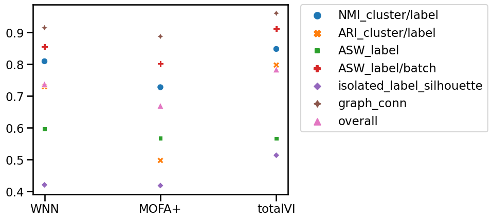
We observe that totalVI obtained the highest overall score, and therefore we will use totalVI embedding later in the notebook to show how one can annotate the cluster in the latent space using both ADT and RNA markers. Depending on the downstream task and the experimental design, selecting the best performing based on a specific metric is advisable.
44.4. Multiome data#
To show that integration methods can also work with multiome (i.e. paired RNA-seq and ATAC-seq) data, we demonstrate how multiVI can be used for this task. We note that WNN and MOFA+ can also be run on multiome data with almost exactly the same code as above, so here we only present multiVI where the underlying model differs from totalVI.
44.4.1. Prepare data#
atac = sc.read(
    "/lustre/groups/ml01/workspace/anastasia.litinetskaya/data/neurips-multiome/atac_hvf.h5ad"
)
atac
AnnData object with n_obs × n_vars = 69249 × 40002
    obs: 'GEX_pct_counts_mt', 'GEX_n_counts', 'GEX_n_genes', 'GEX_size_factors', 'GEX_phase', 'ATAC_nCount_peaks', 'ATAC_atac_fragments', 'ATAC_reads_in_peaks_frac', 'ATAC_blacklist_fraction', 'ATAC_nucleosome_signal', 'cell_type', 'batch', 'ATAC_pseudotime_order', 'GEX_pseudotime_order', 'Samplename', 'Site', 'DonorNumber', 'Modality', 'VendorLot', 'DonorID', 'DonorAge', 'DonorBMI', 'DonorBloodType', 'DonorRace', 'Ethnicity', 'DonorGender', 'QCMeds', 'DonorSmoker', 'cell_type_l2', 'cell_type_l1', 'cell_type_l3', 'assay'
    var: 'feature_types', 'gene_id', 'n_cells', 'prop_shared_cells', 'variability_score'
    uns: 'ATAC_gene_activity_var_names', 'dataset_id', 'genome', 'organism'
    obsm: 'ATAC_gene_activity', 'ATAC_lsi_full', 'ATAC_lsi_red', 'ATAC_umap', 'GEX_X_pca', 'GEX_X_umap'
    layers: 'binary', 'counts', 'cpm', 'tf-idf', 'tf-idf-binary', 'tf-idf-counts'
rna = sc.read(
    "/lustre/groups/ml01/workspace/anastasia.litinetskaya/data/neurips-multiome/rna_hvg.h5ad"
)
rna
AnnData object with n_obs × n_vars = 69249 × 4000
    obs: 'GEX_pct_counts_mt', 'GEX_n_counts', 'GEX_n_genes', 'GEX_size_factors', 'GEX_phase', 'ATAC_nCount_peaks', 'ATAC_atac_fragments', 'ATAC_reads_in_peaks_frac', 'ATAC_blacklist_fraction', 'ATAC_nucleosome_signal', 'cell_type', 'batch', 'ATAC_pseudotime_order', 'GEX_pseudotime_order', 'Samplename', 'Site', 'DonorNumber', 'Modality', 'VendorLot', 'DonorID', 'DonorAge', 'DonorBMI', 'DonorBloodType', 'DonorRace', 'Ethnicity', 'DonorGender', 'QCMeds', 'DonorSmoker'
    var: 'feature_types', 'gene_id', 'highly_variable', 'means', 'dispersions', 'dispersions_norm'
    uns: 'ATAC_gene_activity_var_names', 'Site_colors', 'batch_colors', 'cell_type_colors', 'dataset_id', 'genome', 'hvg', 'organism'
    obsm: 'ATAC_gene_activity', 'ATAC_lsi_full', 'ATAC_lsi_red', 'ATAC_umap', 'GEX_X_pca', 'GEX_X_umap', 'X_umap'
    layers: 'counts'
We again subset the data to one site and 3 batches.
batches_to_keep = ["s1d1", "s1d2", "s1d3"]
rna = rna[rna.obs["batch"].isin(batches_to_keep)]
atac = atac[atac.obs["batch"].isin(batches_to_keep)]
mdata_multiome = mu.MuData({"rna": rna, "atac": atac})
mdata_multiome
MuData object with n_obs × n_vars = 17243 × 44002
  var:	'feature_types', 'gene_id'
  2 modalities
    rna:	17243 x 4000
      obs:	'GEX_pct_counts_mt', 'GEX_n_counts', 'GEX_n_genes', 'GEX_size_factors', 'GEX_phase', 'ATAC_nCount_peaks', 'ATAC_atac_fragments', 'ATAC_reads_in_peaks_frac', 'ATAC_blacklist_fraction', 'ATAC_nucleosome_signal', 'cell_type', 'batch', 'ATAC_pseudotime_order', 'GEX_pseudotime_order', 'Samplename', 'Site', 'DonorNumber', 'Modality', 'VendorLot', 'DonorID', 'DonorAge', 'DonorBMI', 'DonorBloodType', 'DonorRace', 'Ethnicity', 'DonorGender', 'QCMeds', 'DonorSmoker'
      var:	'feature_types', 'gene_id', 'highly_variable', 'means', 'dispersions', 'dispersions_norm'
      uns:	'ATAC_gene_activity_var_names', 'Site_colors', 'batch_colors', 'cell_type_colors', 'dataset_id', 'genome', 'hvg', 'organism'
      obsm:	'ATAC_gene_activity', 'ATAC_lsi_full', 'ATAC_lsi_red', 'ATAC_umap', 'GEX_X_pca', 'GEX_X_umap', 'X_umap'
      layers:	'counts'
    atac:	17243 x 40002
      obs:	'GEX_pct_counts_mt', 'GEX_n_counts', 'GEX_n_genes', 'GEX_size_factors', 'GEX_phase', 'ATAC_nCount_peaks', 'ATAC_atac_fragments', 'ATAC_reads_in_peaks_frac', 'ATAC_blacklist_fraction', 'ATAC_nucleosome_signal', 'cell_type', 'batch', 'ATAC_pseudotime_order', 'GEX_pseudotime_order', 'Samplename', 'Site', 'DonorNumber', 'Modality', 'VendorLot', 'DonorID', 'DonorAge', 'DonorBMI', 'DonorBloodType', 'DonorRace', 'Ethnicity', 'DonorGender', 'QCMeds', 'DonorSmoker', 'cell_type_l2', 'cell_type_l1', 'cell_type_l3', 'assay'
      var:	'feature_types', 'gene_id', 'n_cells', 'prop_shared_cells', 'variability_score'
      uns:	'ATAC_gene_activity_var_names', 'dataset_id', 'genome', 'organism'
      obsm:	'ATAC_gene_activity', 'ATAC_lsi_full', 'ATAC_lsi_red', 'ATAC_umap', 'GEX_X_pca', 'GEX_X_umap'
layers: 'binary', 'counts', 'cpm', 'tf-idf', 'tf-idf-binary', 'tf-idf-counts'mdata_multiome.obs["batch"] = mdata_multiome["rna"].obs["batch"].copy()
mdata_multiome.obs["cell_type"] = mdata_multiome["rna"].obs["cell_type"].copy()
44.4.2. MultiVI#
MultiVI is also based on variational inference and conditional variational autoencoders. The gene expression counts are modeled exactly the same way as in totalVI, i.e. using raw counts and NB distribution. Chromatin accessibility on the other hand is modeled using Bernoulli distribution modeling how likely a particular region is to be open. Hence, the input data for ATAC assay has to be binary where 0 means a closed region and 1 means an open region.
n_genes = len(rna.var_names)
n_regions = len(atac.var_names)
MultiVI requires one AnnData object with concatenated genes and peaks as features. Since we start off with two different objects for each modality but have paired measurements, we can use the following trick to concatenate the AnnData objects along the feature axis.
adata_paired = ad.concat([rna.copy().T, atac.copy().T]).T
adata_paired.obs = adata_paired.obs.join(rna.obs[["cell_type", "batch"]])
adata_paired.obs["modality"] = "paired"
adata_paired
AnnData object with n_obs × n_vars = 17243 × 44002
    obs: 'cell_type', 'batch', 'modality'
    var: 'feature_types', 'gene_id'
    layers: 'counts'
adata_mvi = scvi.data.organize_multiome_anndatas(adata_paired)
We also make sure that we pass raw counts as input to the model by specifying layer='counts' in the setup_anndata function.
scvi.model.MULTIVI.setup_anndata(
    adata_mvi,
    batch_key="modality",
    categorical_covariate_keys=["batch"],
    layer="counts",
)
We initialize the MultiVI model.
mvi = scvi.model.MULTIVI(
    adata_mvi,
    n_genes=n_genes,
    n_regions=n_regions,
)
Next, we train the model with the default parameters.
mvi.train()
GPU available: True (cuda), used: True
TPU available: False, using: 0 TPU cores
IPU available: False, using: 0 IPUs
HPU available: False, using: 0 HPUs
/lustre/groups/ml01/workspace/anastasia.litinetskaya/miniconda3/envs/paired_integration_chapter/lib/python3.9/site-packages/pytorch_lightning/trainer/configuration_validator.py:267: LightningDeprecationWarning: The `Callback.on_epoch_end` hook was deprecated in v1.6 and will be removed in v1.8. Please use `Callback.on_<train/validation/test>_epoch_end` instead.
  rank_zero_deprecation(
LOCAL_RANK: 0 - CUDA_VISIBLE_DEVICES: [0]
Epoch 106/500:  21%|██        | 106/500 [11:30<42:46,  6.51s/it, loss=4.47e+03, v_num=1]
Monitored metric reconstruction_loss_validation did not improve in the last 50 records. Best score: 9223.312. Signaling Trainer to stop.
Finally, we visualize the latent embedding on the UMAP.
mdata_multiome.obsm["X_multiVI"] = mvi.get_latent_representation()
sc.pp.neighbors(mdata_multiome, use_rep="X_multiVI")
sc.tl.umap(mdata_multiome)
mdata_multiome.obsm["X_umap_multiVI"] = mdata_multiome.obsm["X_umap"].copy()
mu.pl.embedding(
    mdata_multiome,
    color=["cell_type", "batch"],
    ncols=1,
    basis="umap_multiVI",
    frameon=False,
)
Session info.
%%R
sessionInfo()
R version 4.2.2 (2022-10-31)
Platform: x86_64-conda-linux-gnu (64-bit)
Running under: CentOS Linux 7 (Core)

Matrix products: default
BLAS/LAPACK: /lustre/groups/ml01/workspace/anastasia.litinetskaya/miniconda3/envs/paired_integration_chapter/lib/libopenblasp-r0.3.21.so

locale:
 [1] LC_CTYPE=C                 LC_NUMERIC=C
 [3] LC_TIME=en_US.UTF-8        LC_COLLATE=en_US.UTF-8
 [5] LC_MONETARY=en_US.UTF-8    LC_MESSAGES=en_US.UTF-8
 [7] LC_PAPER=en_US.UTF-8       LC_NAME=C
 [9] LC_ADDRESS=C               LC_TELEPHONE=C
[11] LC_MEASUREMENT=en_US.UTF-8 LC_IDENTIFICATION=C

attached base packages:
[1] stats4    tools     stats     graphics  grDevices utils     datasets
[8] methods   base

other attached packages:
 [1] Matrix_1.5-3                SingleCellExperiment_1.20.0
 [3] SummarizedExperiment_1.28.0 Biobase_2.58.0
 [5] GenomicRanges_1.50.0        GenomeInfoDb_1.34.1
 [7] IRanges_2.32.0              MatrixGenerics_1.10.0
 [9] matrixStats_0.63.0          S4Vectors_0.36.0
[11] BiocGenerics_0.44.0         SeuratObject_4.1.3
[13] Seurat_4.3.0

loaded via a namespace (and not attached):
  [1] Rtsne_0.16             colorspace_2.0-3       deldir_1.0-6
  [4] ellipsis_0.3.2         ggridges_0.5.4         XVector_0.38.0
  [7] spatstat.data_3.0-0    leiden_0.4.3           listenv_0.9.0
 [10] ggrepel_0.9.2          fansi_1.0.3            codetools_0.2-18
 [13] splines_4.2.2          polyclip_1.10-4        jsonlite_1.8.4
 [16] ica_1.0-3              cluster_2.1.4          png_0.1-8
 [19] uwot_0.1.14            shiny_1.7.4            sctransform_0.3.5
 [22] spatstat.sparse_3.0-0  compiler_4.2.2         httr_1.4.4
 [25] fastmap_1.1.0          lazyeval_0.2.2         cli_3.5.0
 [28] later_1.3.0            htmltools_0.5.4        igraph_1.3.5
 [31] gtable_0.3.1           glue_1.6.2             GenomeInfoDbData_1.2.9
 [34] RANN_2.6.1             reshape2_1.4.4         dplyr_1.0.10
 [37] Rcpp_1.0.9             scattermore_0.8        vctrs_0.5.1
 [40] spatstat.explore_3.0-5 nlme_3.1-161           progressr_0.12.0
 [43] lmtest_0.9-40          spatstat.random_3.0-1  stringr_1.5.0
 [46] globals_0.16.2         mime_0.12              miniUI_0.1.1.1
 [49] lifecycle_1.0.3        irlba_2.3.5.1          goftest_1.2-3
 [52] future_1.30.0          MASS_7.3-58.1          zlibbioc_1.44.0
 [55] zoo_1.8-11             scales_1.2.1           promises_1.2.0.1
 [58] spatstat.utils_3.0-1   parallel_4.2.2         RColorBrewer_1.1-3
 [61] reticulate_1.26        pbapply_1.6-0          gridExtra_2.3
 [64] ggplot2_3.4.0          stringi_1.7.8          rlang_1.0.6
 [67] pkgconfig_2.0.3        bitops_1.0-7           lattice_0.20-45
 [70] ROCR_1.0-11            purrr_1.0.0            tensor_1.5
 [73] patchwork_1.1.2        htmlwidgets_1.6.0      cowplot_1.1.1
 [76] tidyselect_1.2.0       parallelly_1.33.0      RcppAnnoy_0.0.20
 [79] plyr_1.8.8             magrittr_2.0.3         R6_2.5.1
 [82] generics_0.1.3         DelayedArray_0.24.0    pillar_1.8.1
 [85] fitdistrplus_1.1-8     survival_3.4-0         abind_1.4-5
 [88] RCurl_1.98-1.9         sp_1.5-1               tibble_3.1.8
 [91] future.apply_1.10.0    KernSmooth_2.23-20     utf8_1.2.2
 [94] spatstat.geom_3.0-3    plotly_4.10.1          grid_4.2.2
 [97] data.table_1.14.6      digest_0.6.31          xtable_1.8-4
[100] tidyr_1.2.1            httpuv_1.6.7           munsell_0.5.0
[103] viridisLite_0.4.1
44.5. References#
Ricard Argelaguet, Damien Arnol, Danila Bredikhin, Yonatan Deloro, Britta Velten, John C. Marioni, and Oliver Stegle. Mofa+: a statistical framework for comprehensive integration of multi-modal single-cell data. Genome Biology, 21(1):111, May 2020. URL: https://doi.org/10.1186/s13059-020-02015-1, doi:10.1186/s13059-020-02015-1.
Tal Ashuach, Mariano I. Gabitto, Michael I. Jordan, and Nir Yosef. Multivi: deep generative model for the integration of multi-modal data. bioRxiv, 2021. URL: https://www.biorxiv.org/content/early/2021/09/07/2021.08.20.457057, arXiv:https://www.biorxiv.org/content/early/2021/09/07/2021.08.20.457057.full.pdf, doi:10.1101/2021.08.20.457057.
Adam Gayoso, Zoë Steier, Romain Lopez, Jeffrey Regier, Kristopher L. Nazor, Aaron Streets, and Nir Yosef. Joint probabilistic modeling of single-cell multi-omic data with totalvi. Nature Methods, 18(3):272–282, Mar 2021. URL: https://doi.org/10.1038/s41592-020-01050-x, doi:10.1038/s41592-020-01050-x.
Yuhan Hao, Stephanie Hao, Erica Andersen-Nissen, William M. Mauck, Shiwei Zheng, Andrew Butler, Maddie J. Lee, Aaron J. Wilk, Charlotte Darby, Michael Zager, Paul Hoffman, Marlon Stoeckius, Efthymia Papalexi, Eleni P. Mimitou, Jaison Jain, Avi Srivastava, Tim Stuart, Lamar M. Fleming, Bertrand Yeung, Angela J. Rogers, Juliana M. McElrath, Catherine A. Blish, Raphael Gottardo, Peter Smibert, and Rahul Satija. Integrated analysis of multimodal single-cell data. Cell, 184(13):3573–3587.e29, 2021. URL: https://www.sciencedirect.com/science/article/pii/S0092867421005833, doi:https://doi.org/10.1016/j.cell.2021.04.048.
Malte D Luecken, Daniel Bernard Burkhardt, Robrecht Cannoodt, Christopher Lance, Aditi Agrawal, Hananeh Aliee, Ann T Chen, Louise Deconinck, Angela M Detweiler, Alejandro A Granados, Shelly Huynh, Laura Isacco, Yang Joon Kim, Dominik Klein, BONY DE KUMAR, Sunil Kuppasani, Heiko Lickert, Aaron McGeever, Honey Mekonen, Joaquin Caceres Melgarejo, Maurizio Morri, Michaela Müller, Norma Neff, Sheryl Paul, Bastian Rieck, Kaylie Schneider, Scott Steelman, Michael Sterr, Daniel J. Treacy, Alexander Tong, Alexandra-Chloe Villani, Guilin Wang, Jia Yan, Ce Zhang, Angela Oliveira Pisco, Smita Krishnaswamy, Fabian J Theis, and Jonathan M. Bloom. A sandbox for prediction and integration of dna, rna, and proteins in single cells. In Thirty-fifth Conference on Neural Information Processing Systems Datasets and Benchmarks Track (Round 2). 2021. URL: https://openreview.net/forum?id=gN35BGa1Rt.
Malte D. Luecken, M. Büttner, K. Chaichoompu, A. Danese, M. Interlandi, M. F. Mueller, D. C. Strobl, L. Zappia, M. Dugas, M. Colomé-Tatché, and Fabian J. Theis. Benchmarking atlas-level data integration in single-cell genomics. Nature Methods, 19(1):41–50, Jan 2022. URL: https://doi.org/10.1038/s41592-021-01336-8, doi:10.1038/s41592-021-01336-8.
Laura D. Martens, David S. Fischer, Fabian J. Theis, and Julien Gagneur. Modeling fragment counts improves single-cell atac-seq analysis. bioRxiv, 2022. URL: https://www.biorxiv.org/content/early/2022/05/04/2022.05.04.490536, arXiv:https://www.biorxiv.org/content/early/2022/05/04/2022.05.04.490536.full.pdf, doi:10.1101/2022.05.04.490536.
44.6. Contributors#
We gratefully acknowledge the contributions of:
44.6.2. Reviewers#
Lukas Heumos