23. Cell-cell communication#
Key takeaways
Ligand-receptor inference methods and intracellular signaling models (e.g., NicheNet) are complementary approaches for understanding CCC.
Cell-cell communication (CCC) inference from single-cell transcriptomics data relies on the assumption that gene expression is a proxy for protein abundance and intercellular interactions.
Environment setup
Install conda:
Before creating the environment, ensure that conda is installed on your system.
Save the yml content:
Copy the content from the yml tab into a file named
environment.yml.
Create the environment:
Open a terminal or command prompt.
Run the following command:
conda env create -f environment.yml
Activate the environment:
After the environment is created, activate it using:
conda activate <environment_name>
Replace
<environment_name>with the name specified in theenvironment.ymlfile. In the yml file it will look like this:name: <environment_name>
Verify the installation:
Check that the environment was created successfully by running:
conda env list
name: cellcell
channels:
  - conda-forge
  - bioconda
  - r
  - defaults
dependencies:
  - conda-forge::python=3.12.12
  - conda-forge::r-base=4.4.3
  - conda-forge::rpy2=3.6
  - conda-forge::scanpy=1.11.5
  - conda-forge::scikit-misc
  - bioconda::anndata2ri==1.1
  - bioconda::bioconductor-complexheatmap
  - bioconda::bioconductor-limma
  - conda-forge::pip
  - r-seurat
  - r-dplyr
  - r-tidyr
  - r-ggplot2
  - r-purrr
  - r-diagrammer
  - r-mlrmbo
  - r-dicekriging
  - r-hmisc
  - r-remotes
  - r-randomforest
  - r-diffobj
  - r-rstatix
  - r-ggpubr
  - pip:
      - adjusttext==0.7.3
      - decoupler==1.3.3
      - liana==0.1.6
      - mizani==0.8.1
      - palettable==3.3.0
      - plotnine==0.10.1
TL;DR This chapter serves as a brief overview of basic concepts and assumptions of cell-cell communication inference from single-cell transcriptomics data. We provide examples of the two most common approaches for CCC inference: those that focus on ligand-receptor interactions and those that include downstream response.
23.1. Motivation#
Cell communication is a process by which cells react to stimuli from their environment and also from themselves. In multicellular organisms, the dynamic coordination of cells, also called cell-cell communication (CCC), is involved in many biological processes, such as apoptosis and cell migration, and is consequently essential in homeostasis and disease. CCC commonly focuses on protein-mediated interactions, most typically perceived as a secreted ligand binding to its corresponding plasma membrane receptor. However, this picture can be broadened to include secreted enzymes, extra-cellular matrix proteins, transporters, and interactions that require the physical contact between cells, such as cell-cell adhesion proteins and gap junctions [Armingol et al., 2021]. Cell communication is further not independent of other processes, but the contrary, as external stimuli commonly elicit a downstream response. In the case of CCC, this is typically perceived as the induction of canonical pathways and downstream transcription factors in the cells receiving the signal, or receiver cells. Ultimately these external stimuli alter the function of receiver cells, and this alteration is further propagated via the subsequent interaction of these cells with their microenvironment. Traditionally, the study of CCC required specialized in-situ biochemical assays, such as proximity labelling proteomics, co-immunoprecipitation, and yeast two-hybrid screening [Armingol et al., 2021]. Yet, the rapid developments and dropping costs of transcriptomics data generation has enabled a paradigm shift away from focusing on which types of cells are present, but rather on the relationships between them [Almet et al., 2021]. As a consequence, CCC inference from single-cell data is now becoming a routine approach, capable of providing a system-level hypotheses of intercellular crosstalk in vivo.
23.2. Approaches#
As a result of this increased interest, a number of computational tools for CCC inference from single-cell transcriptomics have emerged that can be classified as those that predict CCC interactions alone, commonly referred to as ligand-receptor inference methods (e.g. [Efremova et al., 2020, Hou et al., 2020, Jin et al., 2021, Raredon et al., 2022]), and those that additionally estimate intracellular activities induced by CCC (e.g. [Browaeys et al., 2020, Hu et al., 2021, Wang et al., 2019]). Both categories of tools use gene expression information as a proxy of protein abundance, and typically require the clustering of cells into biologically-meaningful groups (See Annotation tutorial). These CCC tools infer intercellular crosstalk between pairs of cell groups, one group being the source and the other the receiver of a CCC event. CCC events are thus commonly represented as interactions between proteins, expressed by the source and receiver cell clusters.
The information about the interacting proteins is commonly extracted from prior knowledge resources. In the case of ligand-receptor methods, the interactions can also be represented by heteromeric protein complexes, as different subunit combinations can induce distinct responses and the inclusion of protein complex information has been shown to reduce false positive rates [Efremova et al., 2020, Jin et al., 2021, Liu et al., 2022]. On the other hand, the approaches that model intracellular signalling also leverage the functional information in receiver cell types, and thus require additional information such as intracellular protein-protein interaction network and/or gene regulatory interactions.
Recent work has highlighted that the choice of method and/or resource leads to limited consensus in inferred predictions when using different tools [Dimitrov et al., 2022, Liu et al., 2022, Wang et al., 2022], thus prompting caution when interpreting their output. The CCC field is further plagued by the lack of ground truth [Almet et al., 2021, Armingol et al., 2021], capable of capturing the complex and dynamic interplay between large numbers of cells and molecules. Nevertheless, independent evaluations have shown that CCC methods are fairly robust to the introduction of noise [Dimitrov et al., 2022, Liu et al., 2022, Wang et al., 2022], and are largely concordant with alternative data modalities such as intracellular signalling and spatial information [Dimitrov et al., 2022, Liu et al., 2022].
In this chapter, we first provide an introduction and example to perhaps the most common and simplest CCC approaches, i.e. ligand-receptor inference with CellPhoneDB [Efremova et al., 2020] and LIANA [Dimitrov et al., 2022]. Then we showcase NicheNet as an example of a CCC inference method with a focus on intracellular activities downstream of CCC events [Browaeys et al., 2020]. Finally, we highlight the common assumptions and limitations of CCC inference from single-cell transcriptomics data as well as suggestions how to improve confidence in intercellular communication predictions. Note that here we generalize for the sake of simplicity, however, there are a plethora of different and newly emerging CCC approaches. We highlight some of those in the Outlook section.
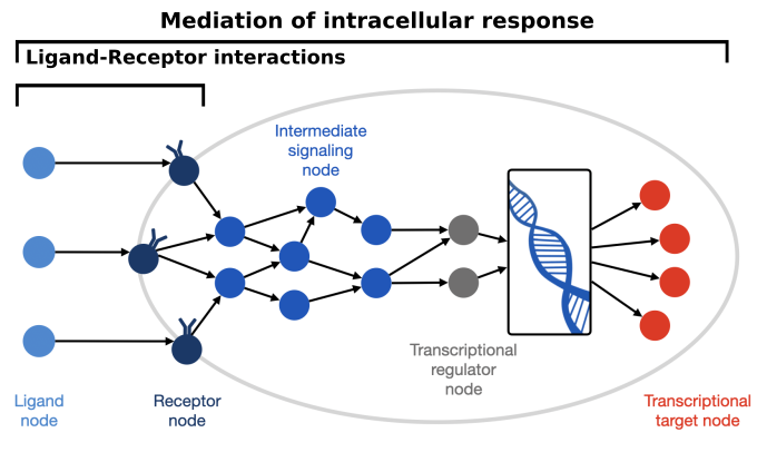
FIGURE 22.1. Cell-Cell Communication Overview
23.3. Environment setup#
# python libs
import decoupler as dc
import liana as li
import matplotlib.pyplot as plt
import numpy as np
import pandas as pd
import scanpy as sc
import seaborn as sns
import session_info
# Setting up R dependencies
import anndata2ri

anndata2ri.activate()

%load_ext rpy2.ipython
%%R
suppressPackageStartupMessages({
    library(reticulate)
    library(ggplot2)
    library(tidyr)
    library(dplyr)
    library(purrr)
    library(tibble)
})
# figure settings
sc.settings.set_figure_params(dpi=200, frameon=False)
sc.set_figure_params(dpi=200, facecolor="white")
sc.set_figure_params(figsize=(5, 5))
23.4. Case Study#
As a simple example, we will look at ~25k PBMCs from 8 lupus patients, each before and after IFN-β stimulation [Kang et al., 2018]. Note that by focusing on PBMCs, for the purpose of this tutorial, we assume that coordinated events occur among them.
So, let’s first download the pre-processed data.
# Read in
adata = sc.read(
    "kang_counts_25k.h5ad", backup_url="https://figshare.com/ndownloader/files/34464122"
)

# Store the counts for later use
adata.layers["counts"] = adata.X.copy()
Apply basic quality control steps to remove any low quality cells and lowly expressed genes. We refer the user to the Quality Control chapter for more extensive QC steps.
sc.pp.filter_cells(adata, min_genes=200)
sc.pp.filter_genes(adata, min_cells=3)
# Store the counts for later use
adata.layers["counts"] = adata.X.copy()
# Rename label to condition, replicate to patient
adata.obs = adata.obs.rename({"label": "condition", "replicate": "patient"}, axis=1)
# assign sample
adata.obs["sample"] = (
    adata.obs["condition"].astype("str") + "&" + adata.obs["patient"].astype("str")
)
We will also normalize the data to ensure that the count depth is equalized for all cells, given that we need the gene expression values to be comparable across the cell types. We refer the user to the Normalization chapter for more information and alternative normalization approaches that might fit their data better.
# log1p normalize the data
sc.pp.normalize_total(adata)
sc.pp.log1p(adata)
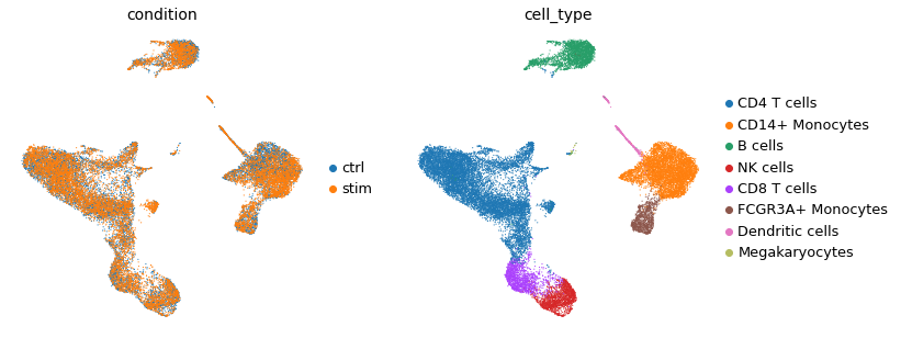
In this case study, we will assume that cell types such as B cells and CD4 T cells carry out a signal mediator role, while others, such as CD8 T cells and Natural Killer cells, are composed of the cells that carry out the response. In other words, we will treat B and CD4 T cells as the sources of CCC signalling, while the latter are the receivers of CCC stimuli. This is of course an oversimplification as signalling sources and receivers are expected to be dynamic and multi-directional, thus the cell types that we treat as which category depends on the hypothesis in mind.
adata.obs["cell_type"].cat.categories
Index(['CD4 T cells', 'CD14+ Monocytes', 'B cells', 'NK cells', 'CD8 T cells',
       'FCGR3A+ Monocytes', 'Dendritic cells', 'Megakaryocytes'],
      dtype='object')
Show pre-computed UMAP, just to showcase the data
sc.pl.umap(adata, color=["condition", "cell_type"], frameon=False)
/home/dbdimitrov/anaconda3/envs/cellcell/lib/python3.10/site-packages/scanpy/plotting/_tools/scatterplots.py:364: UserWarning: No data for colormapping provided via 'c'. Parameters 'cmap' will be ignored
/home/dbdimitrov/anaconda3/envs/cellcell/lib/python3.10/site-packages/scanpy/plotting/_tools/scatterplots.py:364: UserWarning: No data for colormapping provided via 'c'. Parameters 'cmap' will be ignored
23.4.1. Ligand-receptor inference#
First, let’s use the CellPhoneDB (v2) ligand-receptor method [Efremova et al., 2020].
We will run CellPhoneDB on the data post IFN-beta stimulation alone, as such methods were initially designed for the inference of CCC events in “steady-state” data, or in other words, they are meant to be used not across samples or conditions, but rather on a single condition or sample at a time. Note that, nevertheless, certain approaches exist to apply ligand-receptor methods across conditions but these are out of scope for this tutorial, and instead we refer to them in the Outlook section.
adata_stim = adata[adata.obs["condition"] == "stim"].copy()
adata_stim
AnnData object with n_obs × n_vars = 12301 × 15701
    obs: 'nCount_RNA', 'nFeature_RNA', 'tsne1', 'tsne2', 'condition', 'cluster', 'cell_type', 'patient', 'nCount_SCT', 'nFeature_SCT', 'integrated_snn_res.0.4', 'seurat_clusters', 'n_genes', 'sample'
    var: 'name', 'n_cells'
    uns: 'log1p', 'condition_colors', 'cell_type_colors'
    obsm: 'X_pca', 'X_umap'
    layers: 'counts'
# import cellphonedb method via liana
from liana.method import cellphonedb
CellPhoneDB is one of the most commonly-used CCC tools, it represents intercellular communication events as the average gene expression of the proteins involved in the interaction. The proteins involved can also be can also take the form of heteromeric complexes, and in that case the minimum gene expression of the subunits is considered. In addition to the expression average, interaction significance is determined against a null distribution, generated by shuffling the cell group labels.
Note that we are grouping by cell type and that the CCC statistics that we get will reflect the cell types that were previously pre-defined.
cellphonedb(
    adata_stim, groupby="cell_type", use_raw=False, return_all_lrs=True, verbose=True
)
Using `.X`!
Converting mat to CSR format
227 features of mat are empty, they will be removed.
/home/dbdimitrov/anaconda3/envs/cellcell/lib/python3.10/site-packages/pandas/core/indexing.py:1728: ImplicitModificationWarning: Trying to modify attribute `.obs` of view, initializing view as actual.
0.46 of entities in the resource are missing from the data.
Generating ligand-receptor stats for 12301 samples and 15474 features
100%|██████████| 1000/1000 [00:22<00:00, 45.07it/s]
By default, the results are written in place within the anndata object, more specifically in .uns['liana_res'].
Let’s examine the output from the CellPhoneDB method:
adata_stim.uns["liana_res"].head()
| ligand | ligand_complex | ligand_means | ligand_props | receptor | receptor_complex | receptor_means | receptor_props | source | target | lrs_to_keep | lr_means | cellphone_pvals | |
|---|---|---|---|---|---|---|---|---|---|---|---|---|---|
| 0 | LGALS9 | LGALS9 | 0.072739 | 0.101973 | PTPRC | PTPRC | 0.457824 | 0.501761 | CD4 T cells | CD4 T cells | True | 0.265281 | 1.0 |
| 9 | LGALS9 | LGALS9 | 0.072739 | 0.101973 | CD44 | CD44 | 0.304042 | 0.364741 | CD4 T cells | CD4 T cells | True | 0.188391 | 1.0 |
| 37 | VIM | VIM | 0.507059 | 0.519725 | CD44 | CD44 | 0.304042 | 0.364741 | CD4 T cells | CD4 T cells | True | 0.405550 | 1.0 |
| 38 | PKM | PKM | 0.230863 | 0.278267 | CD44 | CD44 | 0.304042 | 0.364741 | CD4 T cells | CD4 T cells | True | 0.267453 | 1.0 |
| 66 | LGALS9 | LGALS9 | 0.072739 | 0.101973 | CD47 | CD47 | 0.213795 | 0.272807 | CD4 T cells | CD4 T cells | True | 0.143267 | 1.0 |
Here, we see that stats are provided for both ligand and receptor entities, more specifically: - ligand and receptor are typically the two entities that interact. As a reminder, CCC events are not limited to secreted signalling, but we refer to them as ligand and receptor for simplicity.
Also, in the case of heteromeric complexes, the ligand and receptor columns represent the subunit with minimum expression, while *_complex corresponds to the actual complex, with subunits being separated by _.
sourceandtargetcolumns represent the source/sender and target/receiver cell identity for each interaction, respectively*_props: represents the proportion of cells that express the entity.By default, in CellPhoneDB and LIANA, any interactions in which either entity is not expressed in above 10% of cells per cell type is considered as a false positive, under the assumption that since CCC occurs between cell types, a sufficient proportion of cells within should express the genes.
*_means: entity expression mean per cell typelr_means: mean ligand-receptor expression, as a measure of ligand-receptor interaction magnitudecellphone_pvals: permutation-based p-values, as a measure of interaction specificity
Note that ligand, receptor, source, and target columns are returned by every ligand-receptor method, while the rest of the columns can vary across the ligand-receptor methods, as each method relies on different assumptions and scoring functions, and hence each returns different ligand-receptor scores.
Nevertheless, typically most methods use a pair of scoring functions - where one often corresponds to the magnitude (strength) of interaction and the other reflects the specificity of a given interaction to a pair of cell identities.
23.4.1.1. Visual exploration#
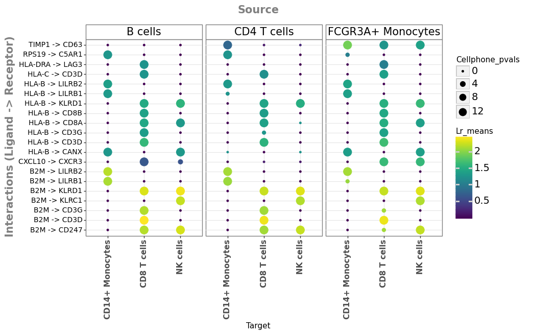
We can now visualize the results that we just obtained as a dotplot, in which rows represent the prioritized interactions between source/sender (top) and target/receiver (bottom) cell types.
li.pl.dotplot(
    adata=adata_stim,
    colour="lr_means",
    size="cellphone_pvals",
    inverse_size=True,  # we inverse sign since we want small p-values to have large sizes
    # We choose only the cell types which we wish to plot
    source_labels=["CD4 T cells", "B cells", "FCGR3A+ Monocytes"],
    target_labels=["CD8 T cells", "CD14+ Monocytes", "NK cells"],
    # since cpdbv2 suggests using a filter to FPs
    # we can filter the interactions according to p-values <= 0.01
    filter_fun=lambda x: x["cellphone_pvals"] <= 0.01,
    # as this type of methods tends to result in large numbers
    # of predictions, we can also further order according to expression magnitude
    orderby="lr_means",
    orderby_ascending=False,  # we want to prioritize those with highest expression
    top_n=20,  # and we want to keep only the top 20 interactions
    figure_size=(9, 5),
    size_range=(1, 6),
)
<ggplot: (8783502753003)>
Great, we get a number of interactions potentially linked to IFN-beta stimulation.
We can also see that both the magnitude (expression strength) and specificity of the interactions are cell-type dependent. For example, the potential binding of HLA-B binding to CD8A/B logically occurs only when the receiver cells are CD8 T cells.
23.4.1.2. Generating a Ligand-Receptor consensus with LIANA#
Given the reported limited agreement between the interactions inferred by different ligand-receptor methods, as a way to further increase the confidence in a potential interaction of interest, one could check if this interaction is predicted as relevant by more than a single method. In the same manner, one could also use multiple methods and focus on their consensus, or in other words focus on interactions consistently predicted as relevant. To this end, we will run the rank_aggregate method of liana [Dimitrov et al., 2022], which generates a probability distribution of highly ranked interactions across the methods.
Let’s first examine the ligand-receptor methods in LIANA:
li.method.show_methods()
| Method Name | Magnitude Score | Specificity Score | Reference | |
|---|---|---|---|---|
| 0 | CellPhoneDB | lr_means | cellphone_pvals | Efremova, M., Vento-Tormo, M., Teichmann, S.A.... |
| 0 | Connectome | expr_prod | scaled_weight | Raredon, M.S.B., Yang, J., Garritano, J., Wang... |
| 0 | log2FC | None | lr_logfc | Dimitrov, D., Türei, D., Garrido-Rodriguez, M.... |
| 0 | NATMI | expr_prod | spec_weight | Hou, R., Denisenko, E., Ong, H.T., Ramilowski,... |
| 0 | SingleCellSignalR | lrscore | None | Cabello-Aguilar, S., Alame, M., Kon-Sun-Tack, ... |
| 0 | CellChat | lr_probs | cellchat_pvals | Jin, S., Guerrero-Juarez, C.F., Zhang, L., Cha... |
| 0 | Rank_Aggregate | magnitude_rank | specificity_rank | Dimitrov, D., Türei, D., Garrido-Rodriguez, M.... |
| 0 | Geometric Mean | lr_gmeans | gmean_pvals | CellPhoneDBv2's permutation approach applied t... |
Let’s now run the Rank_Aggregate method, which will essentially run the other methods in the background and then generate a consensus.
from liana.method import rank_aggregate
rank_aggregate(
    adata_stim, groupby="cell_type", return_all_lrs=True, use_raw=False, verbose=True
)
Using `.X`!
Converting mat to CSR format
227 features of mat are empty, they will be removed.
/home/dbdimitrov/anaconda3/envs/cellcell/lib/python3.10/site-packages/pandas/core/indexing.py:1728: ImplicitModificationWarning: Trying to modify attribute `.obs` of view, initializing view as actual.
0.46 of entities in the resource are missing from the data.
Generating ligand-receptor stats for 12301 samples and 15474 features
Assuming that counts were `natural` log-normalized!
Running CellPhoneDB
100%|██████████| 1000/1000 [00:05<00:00, 171.04it/s]
Running Connectome
Running log2FC
Running NATMI
Running SingleCellSignalR
Running CellChat
100%|██████████| 1000/1000 [01:59<00:00, 8.35it/s]
Let’s now check how the output of liana’s rank_aggregate:
adata_stim.uns["liana_res"].drop_duplicates(
    ["ligand_complex", "receptor_complex"]
).head()
| source | target | ligand_complex | receptor_complex | lr_means | cellphone_pvals | expr_prod | scaled_weight | lr_logfc | spec_weight | lrscore | lr_probs | cellchat_pvals | steady_rank | specificity_rank | magnitude_rank | |
|---|---|---|---|---|---|---|---|---|---|---|---|---|---|---|---|---|
| 1129 | CD8 T cells | CD8 T cells | B2M | CD3D | 2.562213 | 0.0 | 3.070147 | 1.070524 | 0.690730 | 0.062383 | 0.982125 | 0.123504 | 0.0 | 2.092188e-11 | 1.415831e-09 | 9.840017e-13 |
| 831 | CD8 T cells | NK cells | B2M | KLRD1 | 2.511733 | 0.0 | 2.622731 | 1.541763 | 0.858930 | 0.080626 | 0.980689 | 0.110393 | 0.0 | 2.092188e-11 | 1.415831e-09 | 8.965786e-11 |
| 468 | FCGR3A+ Monocytes | CD14+ Monocytes | TIMP1 | CD63 | 1.877567 | 0.0 | 3.374182 | 1.478816 | 1.808744 | 0.123245 | 0.982935 | 0.136754 | 0.0 | 2.092188e-11 | 1.415831e-09 | 9.348292e-09 |
| 1513 | CD8 T cells | FCGR3A+ Monocytes | B2M | LILRB2 | 2.402974 | 0.0 | 1.658766 | 1.466587 | 0.604138 | 0.078486 | 0.975838 | 0.063762 | 0.0 | 2.092188e-11 | 1.415831e-09 | 1.935320e-08 |
| 836 | CD8 T cells | NK cells | B2M | CD247 | 2.414776 | 0.0 | 1.763377 | 1.156763 | 0.644404 | 0.074642 | 0.976548 | 0.041130 | 0.0 | 2.092188e-11 | 1.415831e-09 | 1.228218e-07 |
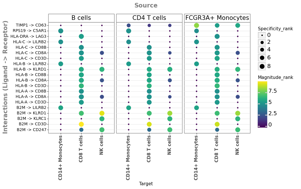
Here, we can see the output of the scoring functions of all methods (refer to the table above, if interested to map which score belong to which method). More importantly, we also get the magnitude_rank and specificity_rank for each interaction, which represent the consensus interaction magnitude (strength of expression) and specificity (across all cell type pairs), respectively. For example, going back to CellPhoneDB, lr_mean and cellphone_pvals will be correspondingly aggregated into those.
Let’s generate the same plot, but now using the aggregate of the methods:
li.pl.dotplot(
    adata=adata_stim,
    colour="magnitude_rank",
    size="specificity_rank",
    inverse_colour=True,  # we inverse sign since we want small p-values to have large sizes
    inverse_size=True,
    # We choose only the cell types which we wish to plot
    source_labels=["CD4 T cells", "B cells", "FCGR3A+ Monocytes"],
    target_labels=["CD8 T cells", "CD14+ Monocytes", "NK cells"],
    # since the rank_aggregate can also be interpreted as a probability distribution
    # we can again filter them according to their specificity significance
    # yet here the interactions are filtered according to
    # how consistently highly-ranked is their specificity across the methods
    # filterby="specificity_rank",
    # filter_lambda=lambda x: x <= 0.05,
    filter_fun=lambda x: x["specificity_rank"] <= 0.05,
    # again, we can also further order according to magnitude
    orderby="magnitude_rank",
    orderby_ascending=True,  # prioritize those with lowest values
    top_n=20,  # and we want to keep only the top 20 interactions
    figure_size=(9, 5),
    size_range=(1, 6),
)
<ggplot: (8783489520283)>
Although, the prioritized interactions by both CellPhoneDB and LIANA seem biologically-plausible and potentially relevant to the treatment, it is challenging to ascertain their relevance. In particular, the advantage of these methods to generate systems-level insights in a hypothesis-free manner happens to also be one of their major disadvantages. Specifically because ligand-receptor tools return all plausible ligand-receptor interactions for every pair of cell types, thus we end up with huge lists of interactions, and choosing targets for subsequent experimental validation can be challenging.
Thus, prior to experimental validation, we suggest that any potential interaction hypotheses should be supported with additional prior knowledge. This may include domain knowledge for the specific condition (e.g. cell types or receptors of interest), as well as orthogonal modalities, such as protein abundance, spatial co-localization, or downstream signalling. To this end, we also further refer the reader to the Gene set enrichment and pathway analysis and spatial CCC (to be added) chapters.
23.4.2. Modelling differential intercellular signalling with NicheNet#
NicheNet is another type of CCC method that considers the intracellular signaling effects triggered by intercellular interactions [Browaeys et al., 2020].
In short, NicheNet infers associations between ligands and the downstream targets that they potentially modulate [Browaeys et al., 2020]. Or in other words, NicheNet assumes that a certain sender/source cell type produces a ligand, and the binding of that ligand to a specific receiver/target cell type(s) leads to a signal propagation that affects master gene regulators, or transcription factors, and subsequently their targets. Therefore, predictions on which target genes are modulated by which ligand-receptor pairs may provide interesting hypotheses concerning the ongoing CCC events. Furthermore, enrichment of target genes of a specific ligand-receptor pair in a receiver cell type can also indicate that this ligand-receptor pair is functionally active. In summary, a NicheNet analysis can thus be performed to 1) infer potential target genes of expressed ligand-receptor interactions and 2) prioritize ligand-receptor interactions based on their target gene enrichment in the receiver. This enrichment is called “ligand activity”, in analogy to transcription factor activity Gene set enrichment and pathway analysis.
To perform these tasks, NicheNet makes use of prior knowledge about ligand-target associations. However, contrary to ligand-receptor databases, comprehensive ligand-target databases do not exist. Therefore, NicheNet predicts ligand-target associations by integrating three layers of prior knowledge covering ligand-receptor, intracellular signaling, and gene regulatory interactions. Using these three layers of information, NicheNet calculates a regulatory potential score for each ligand-target link. This regulatory potential denotes how well prior knowledge supports that a ligand may regulate the expression of a target gene. To calculate regulatory potential, NicheNet first employs a network diffusion algorithm, known as Personalized PageRank (PPR), on the integrated signaling network to estimate the probability that a given ligand may signal to a particular regulator. Specifically, the PPR implementation in NicheNet considers a given ligand as the seed node of interest. Hereby, nodes that are closer to the ligand in the signaling network get higher scores than more distant nodes under the assumption that regulators in the network vicinity of the ligand are more likely modulated by the ligand than more distant nodes. The application of PPR for all ligands in the database thus results in a ligand-regulator matrix of signalling probabilities that are then multiplied with a weight matrix of regulators to target genes in order to obtain ligand-target regulatory potential scores {cite}browaeys_2020. Conceptually, this implies that a ligand–target pair receives a high regulatory potential score if the ligand can signal to regulators of that target gene. These prior knowledge-derived scores are then used in conjunction with the expression data of interacting cells to prioritize ligand-receptor interactions and predict their target genes.
Because NicheNet focuses on how ligands affect gene expression in potentially interacting cells, one needs to be able to define which gene expression changes may (partially) be caused by CCC processes. To rank the ligands according to their potential ligand activity in a receiver cell type, it requires a set of genes assumed to be affected by CCC events in the receiver cell types. The authors of NicheNet recommend ideally defining those sets of genes when working with conditions, e.g. treatment vs control. To this end, we will apply NicheNet in exactly that manner and compare the expression of the patients in our data before and after stimulation with IFN-beta.
For a more detailed description of the NicheNet method, we specifically refer the reader to the footprint part of the Gene set enrichment and pathway analysis chapter as well as NicheNet’s tutorials and manuscript [Browaeys et al., 2020].
23.4.2.1. Load NicheNet Prior-Knowledge#
As mentioned above, NicheNet requires prior knowledge about ligand-receptor interactions and ligand-target links:
a ligand_target_matrix - denotes the potential that a ligand might regulate the expression of a target genes. The weights in this matrix are based on prior knowledge and are required to prioritize possible ligand-receptor interactions and affected target genes.
lr_network - the database of ligand-receptor interactions needed to define expressed ligands, receptors and their interactions.
We will load each of those from Zenodo ![]() (this might take a couple of minutes).
(this might take a couple of minutes).
%%R
# load NicheNet (NicheNet is only available on GitHub)
suppressPackageStartupMessages({
    if(!require(nichenetr)) remotes::install_github("saeyslab/nichenetr", upgrade = "never")
})
%%R
# Increase timeout threshold
options(timeout=600)

# Load PK
ligand_target_matrix <- readRDS(url("https://zenodo.org/record/7074291/files/ligand_target_matrix_nsga2r_final.rds"))
lr_network <- readRDS(url("https://zenodo.org/record/7074291/files/lr_network_human_21122021.rds"))
Moreover, one may also tailor the NicheNet prior knowledge and contextualize the networks according to the data at hand using the OmnipathR package.
23.4.2.1.1. Step 1. Define cell types of interest to be considered as senders/sources and receiver/targets of CCC interactions#
Here, we will assume that multiple cell types are able to affect the receiver cell type
sender_celltypes = ["CD4 T cells", "B cells", "FCGR3A+ Monocytes"]
receiver_celltypes = ["CD8 T cells"]
23.4.2.1.2. Step 2. Define a set of ligands that can potentially affect receiver cell types#
Similarly to the ligand-receptor methods above, here we are only interested in the potential interactions that involve sufficiently expressed genes in each cell type. So, we will assume that e.g. 10% of the cells is a good threshold to reflect genes as expressed within a cell type.
# Helper function to obtain sufficiently expressed genes
from functools import reduce


def get_expressed_genes(adata, cell_type, expr_prop):
    # calculate proportions
    temp = adata[adata.obs["cell_type"] == cell_type, :]
    a = temp.X.getnnz(axis=0) / temp.X.shape[0]
    stats = (
        pd.DataFrame({"genes": temp.var_names, "props": a})
        .assign(cell_type=cell_type)
        .sort_values("genes")
    )

    # obtain expressed genes
    stats = stats[stats["props"] >= expr_prop]
    expressed_genes = stats["genes"].values

    return expressed_genes
sender_expressed = reduce(
    np.union1d,
    [
        get_expressed_genes(adata, cell_type=cell_type, expr_prop=0.1)
        for cell_type in sender_celltypes
    ],
)
receiver_expressed = reduce(
    np.union1d,
    [
        get_expressed_genes(adata, cell_type=cell_type, expr_prop=0.1)
        for cell_type in receiver_celltypes
    ],
)
Then use this information to keep only ligand-receptor pairs in the NicheNet network that are expressed.
%%R -i sender_expressed -i receiver_expressed
# get ligands and receptors in the resource
ligands <- lr_network %>% pull(from) %>% unique()
receptors <- lr_network %>% pull(to) %>% unique()

# only keep the intersect between the resource and the data
expressed_ligands <- intersect(ligands, sender_expressed)
expressed_receptors <- intersect(receptors, receiver_expressed)

# filter the network to only include ligands for which both the ligand and receptor are expressed
potential_ligands <- lr_network %>%
  filter(from %in% expressed_ligands & to %in% expressed_receptors) %>%
  pull(from) %>% unique()
23.4.2.1.3. Step 3. Define a gene set of interest in receiver cell type(s)#
This step is the most critical one in a NicheNet analysis. Here, one defines which genes are potentially modulated by cell-cell communication, i.e. the genes thought to be affected by ligand signalling. For example, one can assume that differentially expressed genes between conditions in receiver cell type(s) are driven by ligands from one of more interacting sender cell populations. Another example would be differentially expressed genes between a differentiated cell population and a progenitor population in case the differentiation is likely induced through interactions with other cell types.
So, we will now use decoupler to generate pseudobulk profiles per cell type and sample, and then perform a differential expression analysis on those. A crucial step of pseudo-bulking is filtering out genes that are not expressed across most cells and samples, since they are very noisy and can result in unstable log-fold changes. To get robust profiles, genes are thus filtered out if again they are not expressed sufficiently per sample (min_prop) and in not enough samples. We refer the reader to the {ref}normalization and {ref}differential-analysis chapters for more info on differential expression analysis and pseudobulk profiles.
# Get pseudo-bulk profile
pdata = dc.get_pseudobulk(
    adata,
    sample_col="sample",
    groups_col="cell_type",
    min_prop=0.1,
    min_smpls=3,
    layer="counts",
)
Normalize the pseudobulk counts
# Storing the raw counts
pdata.layers["counts"] = pdata.X.copy()

# Does PC1 captures a meaningful biological or technical fact?
pdata.obs["lib_size"] = pdata.X.sum(1)

# Normalize
sc.pp.normalize_total(pdata, target_sum=1e4)
sc.pp.log1p(pdata)
# check how this looks like
pdata
AnnData object with n_obs × n_vars = 108 × 4412
    obs: 'condition', 'cell_type', 'patient', 'sample', 'lib_size'
    uns: 'log1p'
    layers: 'counts'
Then we perform a very simple differential analysis contrast. For this example we will use t-test as is implemented in scanpy but we could use any other.
logFCs, pvals = dc.get_contrast(
    pdata,
    group_col="cell_type",
    condition_col="condition",
    condition="stim",
    reference="ctrl",
    method="t-test",
)
Then keep only the positive significant differentially expressed genes in the receiver cell type(s)
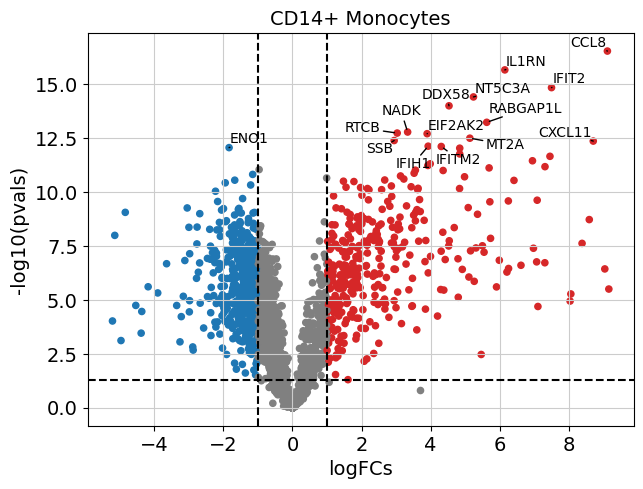
# Visualize those for e.g. CD14+ Monocytes
dc.plot_volcano(logFCs, pvals, "CD14+ Monocytes", top=15, sign_thr=0.05, lFCs_thr=1)
# format results
deg = dc.format_contrast_results(logFCs, pvals)
# only keep the receiver cell type(s)
deg = deg[np.isin(deg["contrast"], receiver_celltypes)]
deg.head()
| contrast | name | logFCs | pvals | adj_pvals | |
|---|---|---|---|---|---|
| 13236 | CD8 T cells | SAMD9L | 3.592979 | 1.818029e-10 | 0.000001 |
| 13237 | CD8 T cells | IFIT3 | 6.486142 | 6.843872e-10 | 0.000002 |
| 13238 | CD8 T cells | IFI6 | 5.555549 | 1.835813e-09 | 0.000003 |
| 13239 | CD8 T cells | OAS1 | 5.479982 | 7.165866e-09 | 0.000008 |
| 13240 | CD8 T cells | IFIT1 | 6.617856 | 1.149598e-08 | 0.00001 |
Now that we have the DE stats for the receiver cell type, we can use those to define the background and geneset of interest for ligand activity analysis with NicheNet.
# define background of sufficiently expressed genes
background_genes = deg["name"].values

# only keep significant and positive DE genes
deg = deg[(deg["pvals"] <= 0.05) & (deg["logFCs"] > 1)]
# get geneset of interest
geneset_oi = deg["name"].values
23.4.2.1.4. Step 4. NicheNet ligand activity estimation#
To estimate ligand activity, NicheNet uses the regulatory potential of genes (based on prior knowledge) to predict which ligand best predicts the gene set of interest. Or in other words, it assesses whether the genes with high regulatory potential in regards to a specific ligand, are more likely to belong to the geneset of interest that we derive for the receiver cell type(s). Conceptually, this is not too dissimilar from standard Gene set enrichment and pathway analysis and NicheNet proposes different ways to estimate ligand activity, such as the area under the receiver operating characteristic curve, or Pearson correlation [Browaeys et al., 2020].
%%R -i geneset_oi -i background_genes -o ligand_activities

ligand_activities <- predict_ligand_activities(geneset = geneset_oi,
                                               background_expressed_genes = background_genes,
                                               ligand_target_matrix = ligand_target_matrix,
                                               potential_ligands = potential_ligands)

ligand_activities <- ligand_activities %>%
  arrange(-aupr) %>%
  mutate(rank = rank(desc(aupr)))

# show top10 ligand activities
head(ligand_activities, n=10)
# A tibble: 10 × 6
   test_ligand auroc   aupr aupr_corrected pearson  rank
   <chr>       <dbl>  <dbl>          <dbl>   <dbl> <dbl>
 1 PTPRC       0.801 0.116          0.0882  0.168      1
 2 HLA-F       0.781 0.104          0.0765  0.188      2
 3 HLA-A       0.776 0.0941         0.0662  0.180      3
 4 HLA-B       0.766 0.0864         0.0586  0.162      4
 5 HLA-E       0.767 0.0856         0.0578  0.129      5
 6 CCL5        0.762 0.0812         0.0534  0.0527     6
 7 CD48        0.762 0.0786         0.0508  0.106      7
 8 B2M         0.753 0.0755         0.0477  0.121      8
 9 HLA-DRA     0.730 0.0694         0.0416  0.111      9
10 CXCL10      0.736 0.0678         0.0400  0.0803    10
23.4.2.1.5. Step 5. Infer & Visualize top-predicted target genes for top ligands#
%%R -o vis_ligand_target
top_ligands <- ligand_activities %>%
  top_n(15, aupr) %>%
  arrange(-aupr) %>%
  pull(test_ligand) %>%
  unique()

# get regulatory potentials
ligand_target_potential <- map(top_ligands,
                               ~get_weighted_ligand_target_links(.x,
                                                                 geneset = geneset_oi,
                                                                 ligand_target_matrix = ligand_target_matrix,
                                                                 n = 500)
                              ) %>%
    bind_rows() %>%
    drop_na()

# prep for visualization
active_ligand_target_links <-
  prepare_ligand_target_visualization(ligand_target_df = ligand_target_potential,
                                      ligand_target_matrix = ligand_target_matrix)

# order ligands & targets
order_ligands <- intersect(top_ligands,
                           colnames(active_ligand_target_links)) %>% rev() %>% make.names()
order_targets <- ligand_target_potential$target %>%
  unique() %>%
  intersect(rownames(active_ligand_target_links)) %>%
  make.names()
rownames(active_ligand_target_links) <- rownames(active_ligand_target_links) %>%
  make.names() # make.names() for heatmap visualization of genes like H2-T23
colnames(active_ligand_target_links) <- colnames(active_ligand_target_links) %>%
  make.names() # make.names() for heatmap visualization of genes like H2-T23

vis_ligand_target <- active_ligand_target_links[order_targets, order_ligands] %>%
  t()

# convert to dataframe, and then it's returned to py
vis_ligand_target <- vis_ligand_target %>%
    as.data.frame() %>%
    rownames_to_column("ligand") %>%
    as_tibble()
# convert dot to underscore and set ligand as index
vis_ligand_target["ligand"] = vis_ligand_target["ligand"].replace(
    r"\.", "_", regex=True
)
vis_ligand_target.set_index("ligand", inplace=True)
# keep only columns where at least one gene has a regulatory potential >= 0.05
vis_ligand_target = vis_ligand_target.loc[
    :, vis_ligand_target[vis_ligand_target >= 0.05].any()
]
vis_ligand_target.head()
| IFI16 | IFIH1 | IFIT2 | IRF7 | MT2A | MX1 | NMI | PARP14 | PARP9 | SOCS1 | TNFSF10 | EPSTI1 | HERC6 | LAP3 | PARP12 | TMEM140 | |
|---|---|---|---|---|---|---|---|---|---|---|---|---|---|---|---|---|
| ligand | ||||||||||||||||
| ICAM1 | 0.010111 | 0.008649 | 0.010065 | 0.013067 | 0.007855 | 0.007761 | 0.000000 | 0.007268 | 0.0000 | 0.008907 | 0.012580 | 0.000000 | 0.000000 | 0.000000 | 0.000000 | 0.00000 |
| CXCL11 | 0.000000 | 0.000000 | 0.000000 | 0.000000 | 0.000000 | 0.000000 | 0.000000 | 0.000000 | 0.0000 | 0.000000 | 0.007285 | 0.000000 | 0.000000 | 0.000000 | 0.000000 | 0.00000 |
| HLA_DQB1 | 0.000000 | 0.000000 | 0.000000 | 0.007094 | 0.000000 | 0.000000 | 0.000000 | 0.000000 | 0.0000 | 0.000000 | 0.007733 | 0.000000 | 0.000000 | 0.000000 | 0.000000 | 0.00000 |
| HMGB1 | 0.158681 | 0.077152 | 0.151255 | 0.091884 | 0.075502 | 0.074791 | 0.147717 | 0.075350 | 0.0745 | 0.078945 | 0.082315 | 0.074556 | 0.073812 | 0.145847 | 0.147686 | 0.07226 |
| ITGB2 | 0.007564 | 0.000000 | 0.006784 | 0.009015 | 0.000000 | 0.000000 | 0.000000 | 0.000000 | 0.0000 | 0.000000 | 0.008748 | 0.000000 | 0.000000 | 0.000000 | 0.000000 | 0.00000 |
23.4.2.1.6. Visualize top ligands & regulatory targets#
fig, ax = plt.subplots(1, 1, figsize=(15, 5))
sns.heatmap(vis_ligand_target, xticklabels=True, ax=ax)
plt.show()
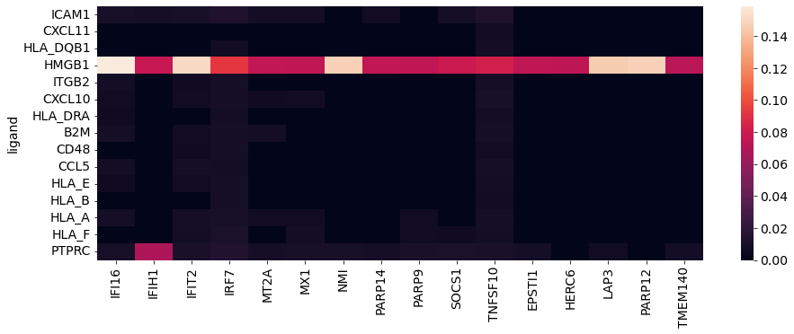
Perfect, we end up with ligands that are most probable to affect downstream signalling in the receiver cell type(s), as well as their most likely targets.
23.4.3. Combining NicheNet output with ligand-receptor inference#
NicheNet and ligand-receptor methods are not exclusive, but rather complementary, as they address different questions and in different ways. Ligand-receptor methods, such as the ones that we show above, infer ligand-receptor interactions using the expression of interacting ligands and receptors, and typically work on “steady-state” data. On the contrary, NicheNet predicts which of these inferred ligand-receptor links are possibly the most functional based on gene expression changes that are induced in the target cell type(s), in a process largely dependent on prior knowledge alone. Thus, while the choice of tool depends on the research question, one could also see ligand-receptor (e.g. CellPhoneDB or LIANA) methods and intracellular signalling CCC methods (e.g. NicheNet) as complementary.
For example, given the top 3 prioritized ligands, we can focus on ligand-receptor pairs that include those and the receiver cell type that we used to infer the active ligands.
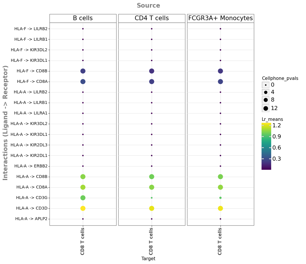
So, let’s see which ligand-receptor interactions that involve the top 5 potentially active ligands from NicheNet were prioritized as consistently relevant by the different methods in LIANA:
ligand_oi = ligand_activities.head(3)["test_ligand"].values
ligand_oi
array(['PTPRC', 'HLA-F', 'HLA-A'], dtype=object)
li.pl.dotplot(
    adata=adata_stim,
    colour="lr_means",
    size="cellphone_pvals",
    inverse_size=True,  # we inverse sign since we want small p-values to have large sizes
    # We choose only the cell types which we wish to plot
    source_labels=sender_celltypes,
    target_labels=receiver_celltypes,
    # keep only those ligands
    # filterby="ligand_complex",
    # filter_lambda=lambda x: np.isin(x, ligand_oi),
    filter_fun=lambda x: x["ligand_complex"] <= 0.01,
    # as this type of methods tends to result in large numbers
    # of predictions, we can also further order according to
    # expression magnitude
    orderby="magnitude_rank",
    orderby_ascending=False,  # we want to prioritize those with highest expression
    top_n=25,  # and we want to keep only the top 25 interactions
    figure_size=(9, 9),
    size_range=(1, 6),
)
<ggplot: (8783461218238)>
From the results, above we can now see the specific ligand-receptor interactions potentially associated with the inferred ligand activities by NicheNet. Moreover, we can hypothesize that the ligand activities inferred by NicheNet, are perhaps affecting the cell types via ligand-receptor interactions specific to some cell type pairs (e.g. HLA-A -> CD3G). Or in other words, while the same ligands may be active as a consequence of IFN-β stimulation, they potentially induce cell-type specific signal transduction changes.
While we use NicheNet and LIANA in this case, some recent CCC tool developments provide various combinations of the ideas and assumptions in these two categories of CCC inference methods (e.g. [Baruzzo et al., 2022, Zhang et al., 2021, Zhang et al., 2021]).
23.5. Key takeaways#
23.5.1. Assumptions & Limitations#
The shared purpose of the methods considered in this work is to predict the most relevant intercellular interactions between different cell types using single-cell transcriptomics data. Thus, all methods assume that the gene expression of different cell types is an informative proxy of the CCC events that occur within the sampled tissue. While single-cell transcriptomics enables the inference of CCC events at a previously unprecedented scale, some assumptions and limitations should be kept in mind. Starting with the assumption that protein co-expressions reflect intercellular interactions, and consequently they are also reflective of any events preceding the interaction, including protein translation and processing, secretion, and diffusion [Armingol et al., 2021, Dimitrov et al., 2022] (Figure 22.2). Furthermore, if cell communication within an organism is conceptualized as the combination of CCC events that occur at different ‘length scales’ or ranges [Palla et al., 2022], then the CCC events that can be inferred from single-cell transcriptomics are potentially limited to only the protein-mediated events that occur at ‘local’ ranges, i.e. between the cell types were sampled. As a result, long-range signalling and CCC driven by other molecules, such as endocrine signalling and system gradients like Calcium and Oxygen concentrations, are likely not captured [Dimitrov et al., 2022].
In addition, while the grouping of cell types according to their lineage is common practice to structure our data, when considering the tissue as the place where communication takes place, interactions do not necessarily occur between cell types but rather individual cells [Wilk et al., 2022]. Also, the intercellular interactions are typically presented as one-to-one events between cell types and/or proteins. Therefore, the assumption that the potential co-expression events across cell types might not necessarily reflect true signalling as in order to fundamentally capture the events within a local community, one must identify the magnitude, directionality and biological relevance of the messages passed between the cells within that community [Armingol et al., 2021].
23.5.2. Summary & Outlook:#
In this chapter we presented two applications of CCC inference methods, namely we used CellPhoneDB and LIANA to predict relevant ligand-receptor interactions from single-context (or steady-state) data and NicheNet to infer potentially active ligands and their targets in a differential-expression context. As the focus of the single-cell field moves further away from the definition of lineages, and into characterizing changes within cell types between conditions, approaches to disentangle CCC insights across contexts are becoming essential. Thus, in addition to NicheNet, we refer the user to other approaches that enable cross-condition comparisons, such as NATMI’s differential cell-connectivity analysis [Hou et al., 2020], Crosstalker’s network topological measures [Nagai et al., 2021], CellChat’s pathway-focused manifold learning [Jin et al., 2021], as well as Tensor-cell2cell’s untargeted factorization approach to infer CCC patterns across contexts [Armingol et al., 2022].
As a consequence of the ongoing developments within the single-cell and the cell-cell communication field specifically, there is an ever-growing number of methods, some of which propose alternative ways to predict CCC events, such as those that work at the single-cell resolution [Raredon et al., 2023, Wang et al., 2019, Wilk et al., 2022]. While others attempt to address some of the limitations above, e.g. by including the inference of interactions mediated by metabolites or small molecules [Garcia-Alonso et al., 2022, Zhang et al., 2021, Zheng et al., 2022].
Albeit, this chapter does not capture the diversity and all current developments of the CCC field in dissociated single-cell data, it serves to highlight some of the general ideas and limitations. Thus, we intend it as a starting point upon which the reader can expand on by combining their knowledge from other chapters, and further reading within the CCC field itself.
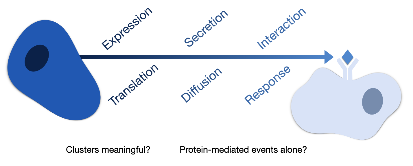
FIGURE 22.2. Assumptions and Limitations of Cell-Cell Communication from single-cell transcriptomics data
23.6. Quiz#
23.7. Contributions#
23.7.2. Reviewers:#
Lukas Heumos
Gregor Sturm
Robin Browaeys
23.8. Session Info#
%%R
sessionInfo()
R version 4.2.2 (2022-10-31)
Platform: x86_64-conda-linux-gnu (64-bit)
Running under: Ubuntu 20.04.5 LTS

Matrix products: default
BLAS/LAPACK: /home/dbdimitrov/anaconda3/envs/cellcell/lib/libopenblasp-r0.3.21.so

locale:
 [1] LC_CTYPE=en_US.UTF-8       LC_NUMERIC=C
 [3] LC_TIME=de_DE.UTF-8        LC_COLLATE=en_US.UTF-8
 [5] LC_MONETARY=de_DE.UTF-8    LC_MESSAGES=en_US.UTF-8
 [7] LC_PAPER=de_DE.UTF-8       LC_NAME=C
 [9] LC_ADDRESS=C               LC_TELEPHONE=C
[11] LC_MEASUREMENT=de_DE.UTF-8 LC_IDENTIFICATION=C

attached base packages:
[1] tools     stats     graphics  grDevices utils     datasets  methods
[8] base

other attached packages:
[1] nichenetr_1.1.1 tibble_3.1.8    purrr_1.0.1     dplyr_1.0.9
[5] tidyr_1.2.0     ggplot2_3.4.0   reticulate_1.25

loaded via a namespace (and not attached):
  [1] backports_1.4.1        circlize_0.4.15        Hmisc_4.7-2
  [4] plyr_1.8.8             igraph_1.3.5           lazyeval_0.2.2
  [7] sp_1.6-0               splines_4.2.2          listenv_0.9.0
 [10] scattermore_0.8        digest_0.6.31          foreach_1.5.2
 [13] htmltools_0.5.4        fansi_1.0.3            checkmate_2.1.0
 [16] magrittr_2.0.3         tensor_1.5             cluster_2.1.4
 [19] doParallel_1.0.17      ROCR_1.0-11            limma_3.54.0
 [22] tzdb_0.3.0             recipes_1.0.4          ComplexHeatmap_2.14.0
 [25] globals_0.16.2         readr_2.1.2            gower_1.0.1
 [28] matrixStats_0.63.0     hardhat_1.2.0          timechange_0.2.0
 [31] spatstat.sparse_3.0-0  jpeg_0.1-10            colorspace_2.0-3
 [34] ggrepel_0.9.2          xfun_0.36              crayon_1.5.2
 [37] jsonlite_1.8.4         progressr_0.13.0       spatstat.data_3.0-0
 [40] survival_3.5-0         zoo_1.8-11             iterators_1.0.14
 [43] glue_1.6.2             polyclip_1.10-4        gtable_0.3.1
 [46] ipred_0.9-13           leiden_0.4.3           GetoptLong_1.0.5
 [49] future.apply_1.10.0    shape_1.4.6            BiocGenerics_0.44.0
 [52] abind_1.4-5            scales_1.2.1           spatstat.random_3.0-1
 [55] miniUI_0.1.1.1         Rcpp_1.0.9             htmlTable_2.4.1
 [58] viridisLite_0.4.1      xtable_1.8-4           clue_0.3-63
 [61] foreign_0.8-84         proxy_0.4-27           Formula_1.2-4
 [64] stats4_4.2.2           lava_1.7.1             prodlim_2019.11.13
 [67] htmlwidgets_1.6.1      httr_1.4.4             DiagrammeR_1.0.9
 [70] RColorBrewer_1.1-3     ellipsis_0.3.2         Seurat_4.3.0
 [73] ica_1.0-3              pkgconfig_2.0.3        nnet_7.3-18
 [76] uwot_0.1.14            deldir_1.0-6           utf8_1.2.2
 [79] caret_6.0-93           tidyselect_1.2.0       rlang_1.0.6
 [82] reshape2_1.4.4         later_1.3.0            visNetwork_2.1.0
 [85] munsell_0.5.0          cli_3.6.0              generics_0.1.3
 [88] ggridges_0.5.4         fdrtool_1.2.17         stringr_1.5.0
 [91] fastmap_1.1.0          goftest_1.2-3          knitr_1.41
 [94] ModelMetrics_1.2.2.2   fitdistrplus_1.1-8     caTools_1.18.2
 [97] randomForest_4.7-1.1   RANN_2.6.1             pbapply_1.7-0
[100] future_1.30.0          nlme_3.1-161           mime_0.12
[103] rstudioapi_0.13        compiler_4.2.2         plotly_4.10.1
[106] png_0.1-8              e1071_1.7-12           spatstat.utils_3.0-1
[109] stringi_1.7.12         lattice_0.20-45        Matrix_1.5-3
[112] vctrs_0.5.1            pillar_1.8.1           lifecycle_1.0.3
[115] spatstat.geom_3.0-3    lmtest_0.9-40          GlobalOptions_0.1.2
[118] RcppAnnoy_0.0.20       bitops_1.0-7           data.table_1.14.6
[121] cowplot_1.1.1          irlba_2.3.5.1          httpuv_1.6.8
[124] patchwork_1.1.2        latticeExtra_0.6-30    R6_2.5.1
[127] promises_1.2.0.1       KernSmooth_2.23-20     gridExtra_2.3
[130] IRanges_2.32.0         parallelly_1.34.0      codetools_0.2-18
[133] MASS_7.3-58.1          rjson_0.2.21           withr_2.5.0
[136] SeuratObject_4.1.3     sctransform_0.3.5      S4Vectors_0.36.0
[139] parallel_4.2.2         hms_1.1.1              grid_4.2.2
[142] rpart_4.1.19           timeDate_4022.108      class_7.3-20
[145] Rtsne_0.16             spatstat.explore_3.0-5 pROC_1.18.0
[148] base64enc_0.1-3        shiny_1.7.4            lubridate_1.9.0
[151] interp_1.1-3
session_info.show()
Click to view session information
-----
anndata             0.8.0
anndata2ri          1.1
decoupler           1.3.3
liana               0.1.6
matplotlib          3.6.3
numpy               1.23.5
pandas              1.5.3
plotnine            0.10.1
rpy2                3.5.7
scanpy              1.7.2
seaborn             0.12.2
session_info        1.0.0
-----
Click to view modules imported as dependencies
PIL                         9.4.0
adjustText                  NA
asttokens                   NA
backcall                    0.2.0
beta_ufunc                  NA
binom_ufunc                 NA
cffi                        1.15.1
colorama                    0.4.6
cycler                      0.10.0
cython_runtime              NA
dateutil                    2.8.2
debugpy                     1.5.1
decorator                   5.1.1
defusedxml                  0.7.1
dunamai                     1.15.0
entrypoints                 0.4
executing                   0.8.3
fontTools                   4.38.0
get_version                 3.5.4
h5py                        3.7.0
hypergeom_ufunc             NA
invgauss_ufunc              NA
ipykernel                   6.9.1
ipython_genutils            0.2.0
ipywidgets                  7.6.5
jedi                        0.18.1
jinja2                      3.1.2
joblib                      1.2.0
kiwisolver                  1.4.4
legacy_api_wrap             0.0.0
llvmlite                    0.39.1
markupsafe                  2.1.2
matplotlib_inline           NA
mizani                      0.8.1
mpl_toolkits                NA
natsort                     8.2.0
nbinom_ufunc                NA
ncf_ufunc                   NA
nct_ufunc                   NA
ncx2_ufunc                  NA
numba                       0.56.4
numexpr                     2.8.3
packaging                   23.0
palettable                  3.3.0
parso                       0.8.3
patsy                       0.5.3
pexpect                     4.8.0
pickleshare                 0.7.5
pkg_resources               NA
prompt_toolkit              3.0.20
ptyprocess                  0.7.0
pure_eval                   0.2.2
pycparser                   2.21
pydev_ipython               NA
pydevconsole                NA
pydevd                      2.6.0
pydevd_concurrency_analyser NA
pydevd_file_utils           NA
pydevd_plugins              NA
pydevd_tracing              NA
pygments                    2.11.2
pyparsing                   3.0.9
pytz                        2022.7.1
pytz_deprecation_shim       NA
scipy                       1.10.0
setuptools                  66.1.1
setuptools_scm              NA
sinfo                       0.3.1
six                         1.16.0
skewnorm_ufunc              NA
sklearn                     1.2.0
stack_data                  0.2.0
statsmodels                 0.13.5
tables                      3.7.0
threadpoolctl               3.1.0
tornado                     6.1
tqdm                        4.64.1
traitlets                   5.1.1
typing_extensions           NA
tzlocal                     NA
wcwidth                     0.2.5
zmq                         23.2.0
zoneinfo                    NA
-----
IPython             8.4.0
jupyter_client      7.2.2
jupyter_core        4.10.0
notebook            6.4.12
-----
Python 3.10.8 | packaged by conda-forge | (main, Nov 22 2022, 08:26:04) [GCC 10.4.0]
Linux-5.15.0-60-generic-x86_64-with-glibc2.31
-----
Session information updated at 2023-02-19 13:46
23.9. References#
Axel A Almet, Zixuan Cang, Suoqin Jin, and Qing Nie. The landscape of cell-cell communication through single-cell transcriptomics. Current Opinion in Systems Biology, 26:12–23, jun 2021. URL: https://linkinghub.elsevier.com/retrieve/pii/S2452310021000081 (visited on 2021-09-06), doi:10.1016/j.coisb.2021.03.007.
Erick Armingol, Hratch M Baghdassarian, Cameron Martino, Araceli Perez-Lopez, Caitlin Aamodt, Rob Knight, and Nathan E Lewis. Context-aware deconvolution of cell-cell communication with tensor-cell2cell. Nature Communications, 13(1):3665, jun 2022. URL: https://www.nature.com/articles/s41467-022-31369-2 (visited on 2021-09-24), doi:10.1038/s41467-022-31369-2.
Erick Armingol, Adam Officer, Olivier Harismendy, and Nathan E Lewis. Deciphering cell-cell interactions and communication from gene expression. Nature Reviews. Genetics, 22(2):71–88, 2021. URL: http://www.nature.com/articles/s41576-020-00292-x (visited on 2021-10-05), doi:10.1038/s41576-020-00292-x.
Giacomo Baruzzo, Giulia Cesaro, and Barbara Di Camillo. Identify, quantify and characterize cellular communication from single-cell rna sequencing data with scseqcomm. Bioinformatics, 38(7):1920–1929, 2022.
Robin Browaeys, Wouter Saelens, and Yvan Saeys. NicheNet: modeling intercellular communication by linking ligands to target genes. Nature Methods, 17(2):159–162, feb 2020. URL: http://www.nature.com/articles/s41592-019-0667-5 (visited on 2021-10-05), doi:10.1038/s41592-019-0667-5.
Daniel Dimitrov, Dénes Türei, Martin Garrido-Rodriguez, Paul L Burmedi, James S Nagai, Charlotte Boys, Ricardo O Ramirez Flores, Hyojin Kim, Bence Szalai, Ivan G Costa, Alberto Valdeolivas, Aurélien Dugourd, and Julio Saez-Rodriguez. Comparison of methods and resources for cell-cell communication inference from single-cell RNA-seq data. Nature Communications, 13(1):3224, jun 2022. URL: https://www.nature.com/articles/s41467-022-30755-0 (visited on 2021-05-31), doi:10.1038/s41467-022-30755-0.
Mirjana Efremova, Miquel Vento-Tormo, Sarah A Teichmann, and Roser Vento-Tormo. CellPhoneDB: inferring cell-cell communication from combined expression of multi-subunit ligand-receptor complexes. Nature Protocols, 15(4):1484–1506, apr 2020. URL: http://www.nature.com/articles/s41596-020-0292-x (visited on 2020-12-04), doi:10.1038/s41596-020-0292-x.
Luz Garcia-Alonso, Valentina Lorenzi, Cecilia Icoresi Mazzeo, João Pedro Alves-Lopes, Kenny Roberts, Carmen Sancho-Serra, Justin Engelbert, Magda Marečková, Wolfram H Gruhn, Rachel A Botting, Tong Li, Berta Crespo, Stijn van Dongen, Vladimir Yu Kiselev, Elena Prigmore, Mary Herbert, Ashley Moffett, Alain Chédotal, Omer Ali Bayraktar, Azim Surani, Muzlifah Haniffa, and Roser Vento-Tormo. Single-cell roadmap of human gonadal development. Nature, 607(7919):540–547, jul 2022. URL: https://www.nature.com/articles/s41586-022-04918-4 (visited on 2022-07-07), doi:10.1038/s41586-022-04918-4.
Rui Hou, Elena Denisenko, Huan Ting Ong, Jordan A Ramilowski, and Alistair RR Forrest. Predicting cell-to-cell communication networks using natmi. Nature communications, 11(1):1–11, 2020.
Yuxuan Hu, Tao Peng, Lin Gao, and Kai Tan. CytoTalk: de novo construction of signal transduction networks using single-cell transcriptomic data. Science Advances, apr 2021. URL: https://advances.sciencemag.org/lookup/doi/10.1126/sciadv.abf1356 (visited on 2021-10-11), doi:10.1126/sciadv.abf1356.
Suoqin Jin, Christian F Guerrero-Juarez, Lihua Zhang, Ivan Chang, Raul Ramos, Chen-Hsiang Kuan, Peggy Myung, Maksim V Plikus, and Qing Nie. Inference and analysis of cell-cell communication using CellChat. Nature Communications, 12(1):1088, feb 2021. URL: http://dx.doi.org/10.1038/s41467-021-21246-9 (visited on 2021-10-05), doi:10.1038/s41467-021-21246-9.
Hyun Min Kang, Meena Subramaniam, Sasha Targ, Michelle Nguyen, Lenka Maliskova, Elizabeth McCarthy, Eunice Wan, Simon Wong, Lauren Byrnes, Cristina M Lanata, and others. Multiplexed droplet single-cell rna-sequencing using natural genetic variation. Nature biotechnology, 36(1):89–94, 2018.
Zhaoyang Liu, Dongqing Sun, and Chenfei Wang. Evaluation of cell-cell interaction methods by integrating single-cell RNA sequencing data with spatial information. Genome Biology, 23(1):218, oct 2022. URL: http://dx.doi.org/10.1186/s13059-022-02783-y (visited on 2022-10-20), doi:10.1186/s13059-022-02783-y.
James S Nagai, Nils B Leimkühler, Michael T Schaub, Rebekka K Schneider, and Ivan G Costa. Crosstalker: analysis and visualization of ligand–receptorne tworks. Bioinformatics, 37(22):4263–4265, 2021.
Giovanni Palla, David S Fischer, Aviv Regev, and Fabian J Theis. Spatial components of molecular tissue biology. Nature Biotechnology, 40(3):308–318, 2022.
Micha Sam Brickman Raredon, Junchen Yang, James Garritano, Meng Wang, Dan Kushnir, Jonas Christian Schupp, Taylor S Adams, Allison M Greaney, Katherine L Leiby, Naftali Kaminski, Yuval Kluger, Andre Levchenko, and Laura E Niklason. Computation and visualization of cell-cell signaling topologies in single-cell systems data using connectome. Scientific Reports, 12(1):4187, mar 2022. URL: http://dx.doi.org/10.1038/s41598-022-07959-x (visited on 2021-01-25), doi:10.1038/s41598-022-07959-x.
Micha Sam Brickman Raredon, Junchen Yang, Neeharika Kothapalli, Wesley Lewis, Naftali Kaminski, Laura E Niklason, and Yuval Kluger. Comprehensive visualization of cell-cell interactions in single-cell and spatial transcriptomics with NICHES. Bioinformatics, jan 2023. URL: http://dx.doi.org/10.1093/bioinformatics/btac775 (visited on 2022-01-27), doi:10.1093/bioinformatics/btac775.
Saidi Wang, Hansi Zheng, James S Choi, Jae K Lee, Xiaoman Li, and Haiyan Hu. A systematic evaluation of the computational tools for ligand-receptor-based cell-cell interaction inference. Briefings in functional genomics, 21(5):339–356, sep 2022. URL: http://dx.doi.org/10.1093/bfgp/elac019 (visited on 2022-04-27), doi:10.1093/bfgp/elac019.
Shuxiong Wang, Matthew Karikomi, Adam L MacLean, and Qing Nie. Cell lineage and communication network inference via optimization for single-cell transcriptomics. Nucleic Acids Research, 47(11):e66, jun 2019. URL: https://academic.oup.com/nar/article/47/11/e66/5421812 (visited on 2019-05-01), doi:10.1093/nar/gkz204.
Aaron J Wilk, Alex K Shalek, Susan Holmes, and Catherine A Blish. Comparative analysis of cell-cell communication at single-cell resolution. BioRxiv, mar 2022. URL: http://biorxiv.org/lookup/doi/10.1101/2022.02.04.479209 (visited on 2022-02-22), doi:10.1101/2022.02.04.479209.
Yang Zhang, Tianyuan Liu, Xuesong Hu, Mei Wang, Jing Wang, Bohao Zou, Puwen Tan, Tianyu Cui, Yiying Dou, Lin Ning, and others. Cellcall: integrating paired ligand–receptor and transcription factor activities for cell–cell communication. Nucleic Acids Research, 49(15):8520–8534, 2021.
Yang Zhang, Tianyuan Liu, Jing Wang, Bohao Zou, Le Li, Linhui Yao, Kechen Chen, Lin Ning, Bingyi Wu, Xiaoyang Zhao, and others. Cellinker: a platform of ligand–receptor interactions for intercellular communication analysis. Bioinformatics, 37(14):2025–2032, 2021.
Yang Zhang, Tianyuan Liu, Jing Wang, Bohao Zou, Le Li, Linhui Yao, Kechen Chen, Lin Ning, Bingyi Wu, Xiaoyang Zhao, and Dong Wang. Cellinker: a platform of ligand-receptor interactions for intercellular communication analysis. Bioinformatics, jan 2021. URL: http://dx.doi.org/10.1093/bioinformatics/btab036 (visited on 2021-09-12), doi:10.1093/bioinformatics/btab036.
Rongbin Zheng, Yang Zhang, Tadataka Tsuji, Lili Zhang, Yu-Hua Tseng, and Kaifu Chen. MEBOCOST: metabolic cell-cell communication modeling by single cell transcriptome. BioRxiv, may 2022. URL: http://biorxiv.org/lookup/doi/10.1101/2022.05.30.494067 (visited on 2022-06-02), doi:10.1101/2022.05.30.494067.