31. Imputation

31.1. Motivation

Unlike spot-based spatial transcriptomics, targeted in-situ technologies (such as MERFISH, smFISH, or seqFISH+) are not limited in their spatial resolution but gene throughput, typically limited to a few hundreds of preselected genes. As a consequence, we face the orthogonal problem of increasing resolution with respect to genes instead of increasing spatial resolution and identifying cellular features. Hence, we would like to impute genes that are measured in scRNA-seq but not in FISH-based technologies.

31.2. Constructing a map between technologies

A method that is widely applicable in the context of aligning spatial profiling measurements with common sc/snRNA-seq profiles is Tangram[Biancalani et al., 2021]. An independent benchmark[Li et al., 2022] showed that Tangram outperformed other imputation methods like gimVI[Lopez et al., 2019] and SpaGE[Abdelaal et al., 2020] in terms of different accuracy metrics and scalability. While Tangram can also be applied in the previously described deconvolution context, we focus on its ability to map MERFISH data to whole genome expression profiles. The underlying idea of Tangram is the probabilistic alignment of two different technologies by means of a single shared modality, typically RNA-seq data. This way, limitations with respect to the number of genes that are measured or spatial resolution can be overcome.

The mapping algorithm of Tangram builds on count matrices from the two technologies at hand. For sc/snRNa-seq data, this means to compute the matrix \(S\) whose entry \(S_{ik}\) indicates the expression level for cell \(i\) and gene \(k\):

\[S \in \mathbb{R}_+^{n_{\text{cells}}\times n_{\text{genes}}} \ \ \text{ with } \ \ S_{ik}>0 \quad . \]

The same procedure applies to spatial data. We build the matrix \(G\) according to:

\[ G \in \mathbb{R}_+^{n_{\text{voxels}}\times n_{\text{genes}}} \ \ \text{ with } \ \ G_{jk}>0 \]

For MERFISH data, a voxel means the aggregation of single gene measurements to individual cells while a voxels refers to the individual spots for Visium. Note that the specific order in the voxel dimension is arbitrary and that \(n_{genes}\) corresponds to the shared subset of genes present in both technologies.

Tangram makes further use of a voxel density vector \(\textbf d\). This density corresponds to estimated cell densities which, for example, can be deduced from an image segmentation in the case of Visium data. Formally, we write:

\[ \textbf{d} \in \mathbb{R}^{n_\text{voxels}} \ \ \text{ with } \ \ d_j \in [0,1] \ \ \text{ and } \ \ \sum_j d_j = 1 \quad . \]

Given the matrices \(S\) and \(G\) as well as the density \(\textbf d\), Tangram aims to learn a thrid matrix \(M\) that expresses the probability \(M_{ij} \in [0,1]\) that cell \(i\) belongs to voxel \(j\). Being probabilistic, every cell has to be mapped exactly once, that is the rows of \(M\) have to be normalised:

\[ M \in \mathbb{R}^{n_{\text{cells}}\times n_{\text{voxels}}}_+ \ \ \text{ with } \ \ \sum_{j}^{n_\text{voxel}} M_{ij}=1 \quad . \]

Note that the sum across cells indicates the number of cells that are assigned to a voxel \(j\). Knowing about the number of cells in \(S\), we can estimate the voxel density as

\[ m_j = \sum_{i}^{n_\text{cells}} \frac{M_{ij}}{n_\text{cells}} \quad . \]

Putting all parts together, we arrive at the objective function of Tangram:

\[ L = \mathbb{KL}[\mathbf m, \mathbf d] - \sum_{k}^{n_\text{genes}} d_{\cos}(M^TS_{:k}, G_{:k}) - \sum_{j}^{n_\text{voxels}} d_{\cos}(M^TS_{j:}, G_{j:}) \quad , \]

where \(M^TS\) is the predicted spatial gene expression, \(\mathbb{KL}\) the Kullback-Leibler divergence and \(d_{\cos}\) the cosine similarity. The first term matches the predicted voxel density \(\textbf m\) with the estimated one \(\textbf d\). The second term ensures that for each gene \(k\) the predicted profile matches the expected profile from \(G\). The third term serves the same purpose for each individual voxel: the predicted voxel expression should be close to the expected one from \(G\).

In order to infer genome-scale expression maps for MERFISH data, we first identify the shared gene set which should result in about \(\sim 200\) genes. Second, we compute the \(S\) and \(G\) matrices from the sc/scRNA-seq reference and the spatial assay, respectively. For MERFISH, the voxel density has uniform entries \(1/n_{\text{voxels}}\) as the voxels correspond to cells themselves. Given this, we only have to optimise the objective \(L\) and obtain the probabilistic mapping \(M\).

To infer the spatial expression for the whole genome \(f_j\) for voxel \(j\), one can either compute a weighted sum using the probabilistic cell assignments \(f_j = \sum_i M_{ij} c_i\), where \(c_i \in \mathbb{R}_+^{n'_\text{genes}}\) is the genome-wide expression profile from sc/snRNA-seq, or first compute a deterministic mapping via \(i^*(j) = \arg\max_i M_{ij}\) and then build the genome-scale profile as \(f_j = c_{i^*(j)}\) .

31.3. Using Tangram in practise

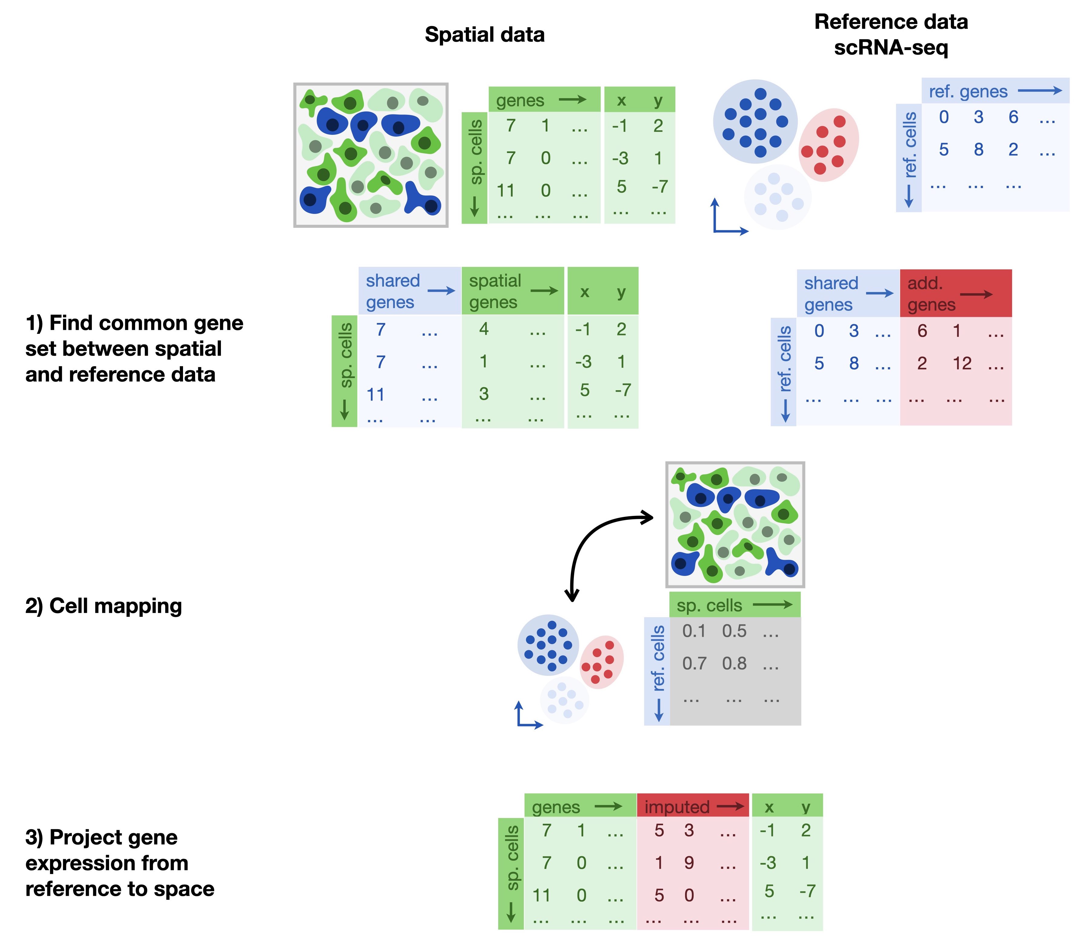
Fig. 31.1 Imputation methods leverage a whole transcriptome reference dataset to map cells onto space. Tangram learns a mapping matrix between the reference and the spatial dataset on the common gene set.

Before we enter this notebook’s analysis, let’s set up our environment.

import scanpy as sc
import tangram as tg
import seaborn as sns
import pandas as pd

import matplotlib.pyplot as plt
from sklearn.preprocessing import MinMaxScaler

sc.settings.verbosity = 3
sc.settings.set_figure_params(dpi=80, facecolor="white")

The dataset used in this tutorial was measured by multiplexed error robust fluorescence in situ hybridization (MERFISH) and investigates the spatial organization and transcriptional profile of wild type hematopoietic stem cell (HSC) niches in fetal liver[Lu et al., 2021]. The dataset contains 140 images across four fetal livers at E14.5 with 132 genes observed in 40,864 cells. Lu et al.[Lu et al., 2021] additionally performed single-cell RNA sequencing of E14.5 whole fetal liver cells by 10x Genomics platform, which we will use as a whole transcriptome reference for this tutorial.

We will first load the reference dataset.

adata_sc = sc.read(
    filename="lu_scRNA_mouse_fetal_liver_2021.h5ad",
    backup_url="https://figshare.com/ndownloader/files/39360860",
)
adata_sc

AnnData object with n_obs × n_vars = 9448 × 28692
    var: 'chozen_isoform', 'code'

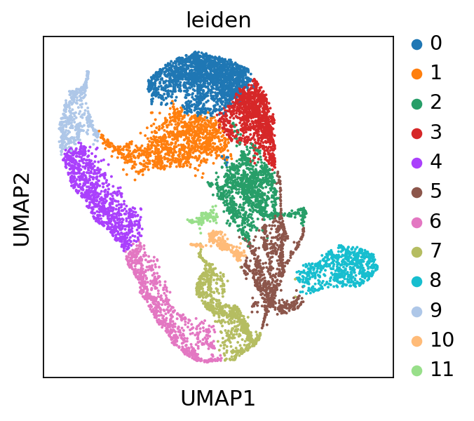
The single-cell RNA-seq reference we are using to showcase the usage of Tangram is not annotated. We therefore apply a basic processing to obtain leiden clusters which we can later project onto the spatial dataset.

sc.pp.neighbors(adata_sc)
sc.tl.leiden(adata_sc, resolution=0.25)
sc.tl.umap(adata_sc)
sc.pl.umap(adata_sc, color="leiden")

computing neighbors
WARNING: You’re trying to run this on 28692 dimensions of `.X`, if you really want this, set `use_rep='X'`.
         Falling back to preprocessing with `sc.pp.pca` and default params.
computing PCA
    with n_comps=50
    finished (0:00:19)
    finished: added to `.uns['neighbors']`
    `.obsp['distances']`, distances for each pair of neighbors
    `.obsp['connectivities']`, weighted adjacency matrix (0:00:35)
running Leiden clustering
    finished: found 12 clusters and added
    'leiden', the cluster labels (adata.obs, categorical) (0:00:00)
computing UMAP
    finished: added
    'X_umap', UMAP coordinates (adata.obsm) (0:00:18)

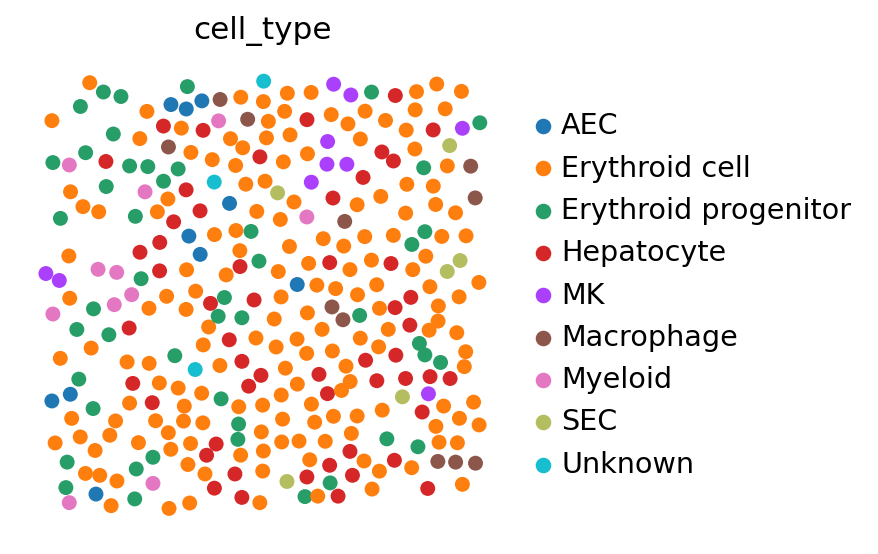
Next, we load the spatial transcriptomics dataset. The MERFISH dataset contains data from X different field of views (FOV).

adata_st = sc.read(
    filename="lu_merfish_mouse_fetal_liver_2021.h5ad",
    backup_url="https://figshare.com/ndownloader/files/39360836",
)
adata_st

AnnData object with n_obs × n_vars = 40864 × 132
    obs: 'CellID', 'FOV', 'CellTypeID_new', 'cell_type'
    obsm: 'spatial'

sc.pl.spatial(
    adata_st[adata_st.obs.FOV == 0], color="cell_type", spot_size=50, frameon=False
)

31.3.1. Common gene set between reference and spatial dataset

We want to select our training genes. These genes are shared between the two datasets and should capture the biological variance between cell types. For this, we first compute marker genes on the single-cell data and then use Tangram’s preprocessing function to subset to those genes that are also present in the spatial data.

markers = list(set.intersection(set(adata_sc.var_names), set(adata_st.var_names)))
len(markers)

132

tg.pp_adatas does the following:

• Computes the overlap between single-cell data and spatial data on the list of genes provided in the genes argument

• Stores the resulting gene set under 'training_genes' in both adata objects under the .uns key

• Enforces consistent ordering of the genes

• To reduce potential naming errors gene names are converted to lower case. To prevent this behaviour set gene_to_lowercase = False.

tg.pp_adatas(adata_sc, adata_st, genes=markers)

filtered out 10726 genes that are detected in less than 1 cells

INFO:root:132 training genes are saved in `uns``training_genes` of both single cell and spatial Anndatas.
INFO:root:132 overlapped genes are saved in `uns``overlap_genes` of both single cell and spatial Anndatas.
INFO:root:uniform based density prior is calculated and saved in `obs``uniform_density` of the spatial Anndata.
INFO:root:rna count based density prior is calculated and saved in `obs``rna_count_based_density` of the spatial Anndata.

Let us check that the function performs as we expect:

assert "training_genes" in adata_sc.uns
assert "training_genes" in adata_st.uns

print(f"Number of training_genes: {len(adata_sc.uns['training_genes'])}")

Number of training_genes: 132

31.3.2. Computing the map from single-cells to spatial voxels

Having specified the training genes, we can now create the map from dissociated single-cell measurements to the spatial locations. For this, we are going to use the map_cells_to_space function from tangram. This function has two different modes, mode='cells' and mode='clusters'. The latter only maps averaged single-cells which makes the mapping computationally faster and more robust when mapping between specimen. However, as we are interested in imputing our spatial data, we will rely on the cell mode which might require access to a GPU for reasonable runtime.

ad_map = tg.map_cells_to_space(
    adata_sc,
    adata_st,
    mode="cells",
    density_prior="rna_count_based",
    num_epochs=500,
    device="cuda",  # or: cpu
)

INFO:root:Allocate tensors for mapping.
INFO:root:Begin training with 132 genes and rna_count_based density_prior in cells mode...
INFO:root:Printing scores every 100 epochs.

Score: 0.271, KL reg: 0.346
Score: 0.911, KL reg: 0.005
Score: 0.931, KL reg: 0.002
Score: 0.937, KL reg: 0.002
Score: 0.941, KL reg: 0.001

INFO:root:Saving results..

The resulting ad_map is itself an AnnData object. Let us inspect it:

ad_map

AnnData object with n_obs × n_vars = 9448 × 40864
    obs: 'leiden'
    var: 'CellID', 'FOV', 'CellTypeID_new', 'cell_type', 'uniform_density', 'rna_count_based_density'
    uns: 'train_genes_df', 'training_history'

We observe that Tangram’s mapping from cell i to spatial voxels j is stored in the .X property of ad_map.

Hence, the meaning of the .var and .obs also changes:

• in .var we have the available metadata of the spatial data, adata_st

• in .obs we have the available metadata of the single-cell data, adata_sc

In addition, the information about the training run is stored in the .uns key, see .uns['training_genes_df'] and .uns[training_history].

31.3.3. Imputing genes and mapping cell-types to space

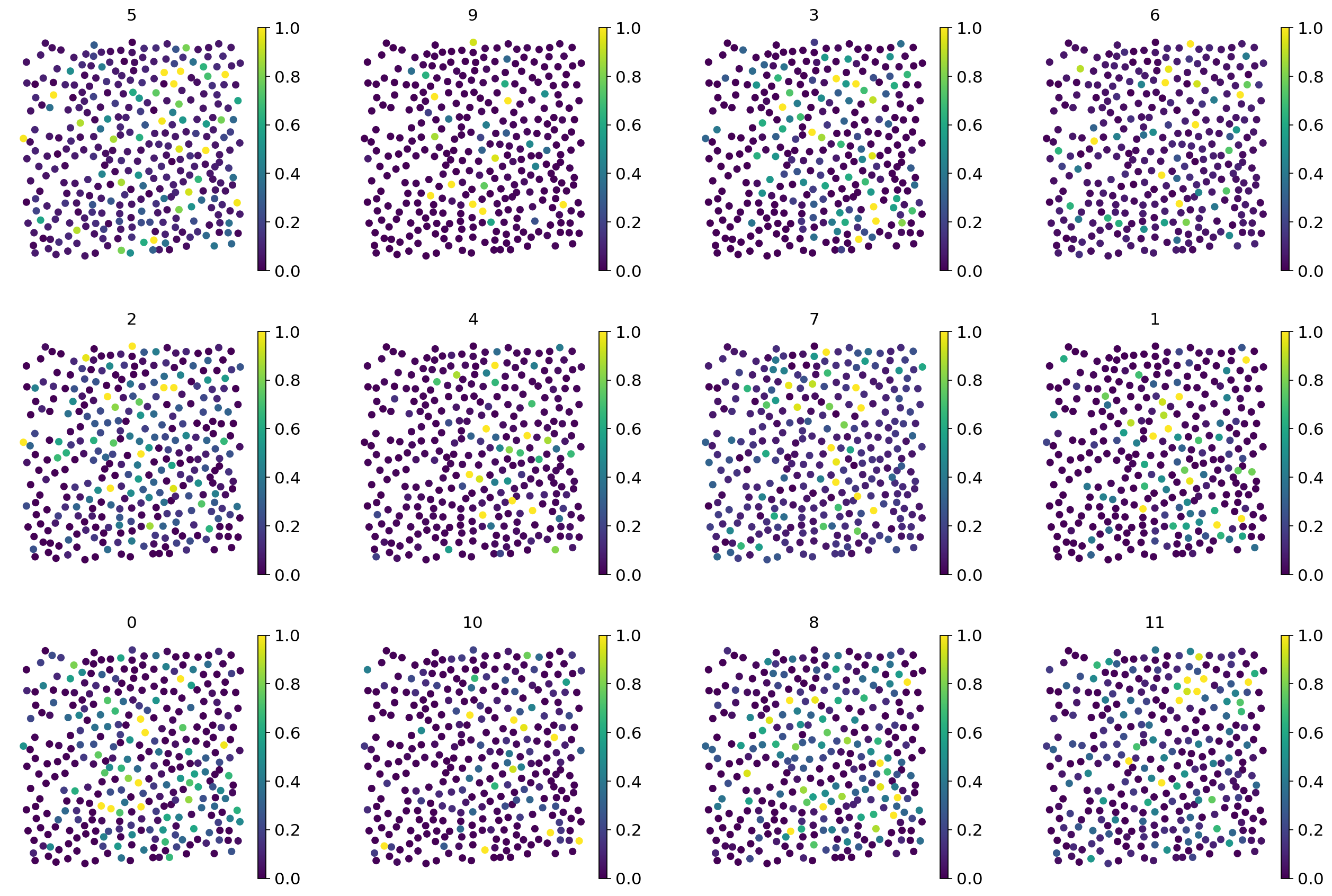
We can use this result in two ways. First, we can map the cell type information that was originally only present in the single-cell data to space. This an easy way to check that your results are biologically consistent by looking for known cell type patterns. Second, we can investigate the spatial gene-expression of those genes that have not been measured with the in-situ method in the first place, effectively imputing all the missing genes.

# Project the cell annotation to spatial locations
tg.project_cell_annotations(ad_map, adata_st, annotation="leiden")
annotation_list = list(pd.unique(adata_sc.obs["leiden"]))

# Plot the spatial annotation
# The `perc` argument steers the range of the colourmap and can help with removing outliers.
tg.plot_cell_annotation_sc(
    adata_st[adata_st.obs.FOV == 0], annotation_list, perc=0.02, spot_size=50
)

INFO:root:spatial prediction dataframe is saved in `obsm` `tangram_ct_pred` of the spatial AnnData.

#  To get a deeper sense, Tangram also computes several scores, which are readily plotted
tg.plot_training_scores(ad_map, bins=20, alpha=0.5)

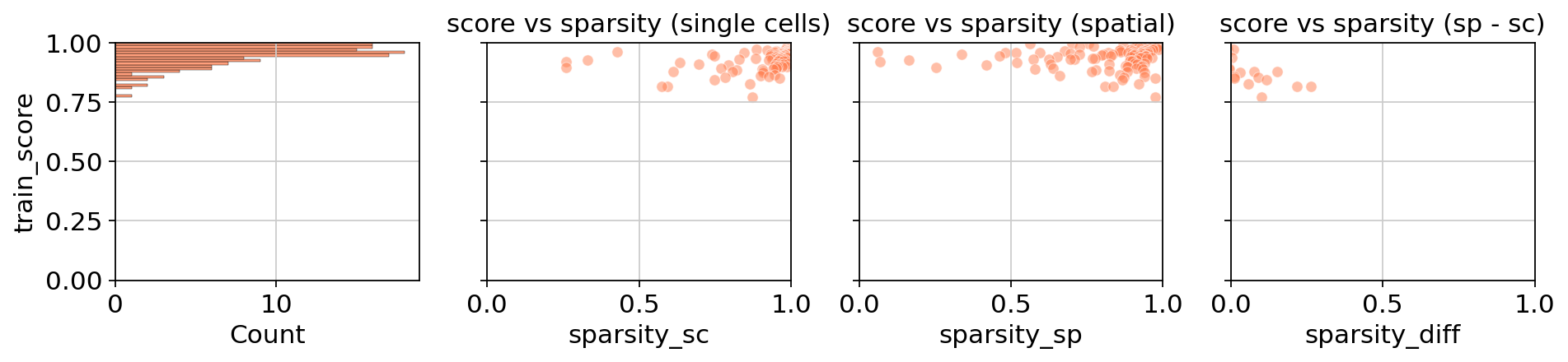
The score generally measures the similarity between original measurement (by the spatial technology) and the inferred mapping by single-cell data. The middle panels both relate the sparsity of the respective data, single-cell and spatial, of a training genes (each dot is a training gene) with the achieved score. As you can see, the performance is much more correlated with the spatial data which is often more sparse and therefore responsible for low-quality mappings. The last panel sets both technologies in context. Genes that have similar sparsity levels in both spatial and single-cell data usually achieve better scores than those that are inconsistent across technologies.

Minor remark: The similarity that Tangram builds on is cosine similarity.

Even more detailed information can be found in the .uns["train_genes_df"].

Now, we can project the genes present in the single-cell data to the spatial locations. This is easily achieved by multiplying the mapping matrix stored in ad_map with the original single-cell data stored in adata_sc. Tangram already provides a convenience function which takes in a mapping and the corresponding single-cell data. The result is a spatial voxel by genes matrix which technically is identical to the original spatial data adata_st but contains expression values for all genes.

ad_ge = tg.project_genes(adata_map=ad_map, adata_sc=adata_sc)
ad_ge

AnnData object with n_obs × n_vars = 40864 × 17966
    obs: 'CellID', 'FOV', 'CellTypeID_new', 'cell_type', 'uniform_density', 'rna_count_based_density'
    var: 'chozen_isoform', 'code', 'n_cells', 'sparsity', 'is_training'
    uns: 'neighbors', 'leiden', 'umap', 'leiden_colors', 'training_genes', 'overlap_genes'

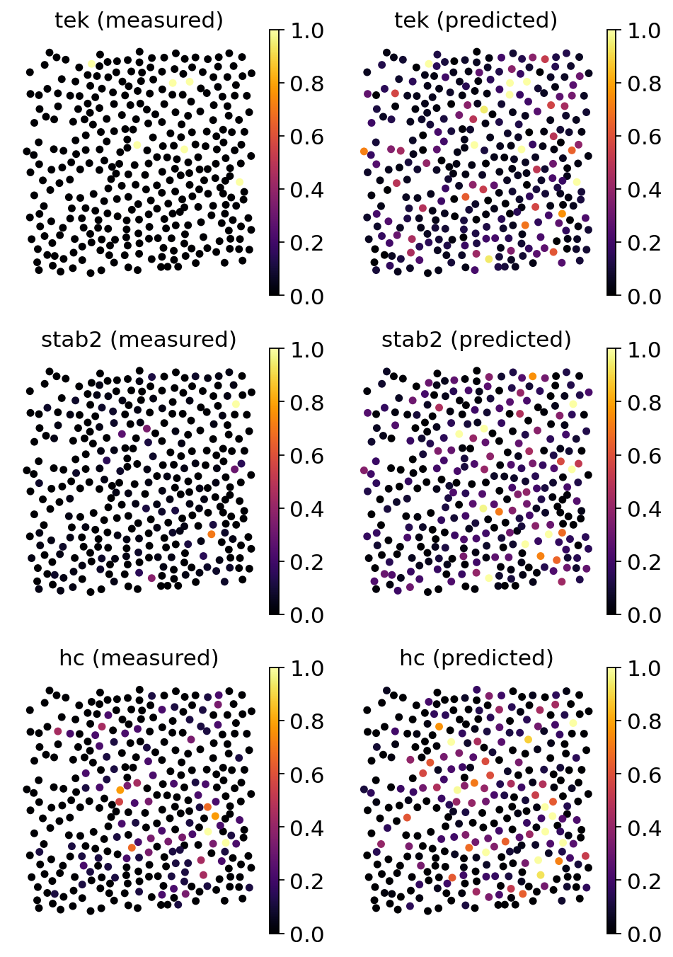
Next, we will compare the new spatial data with the originial measurements. This will provide us with a better feeling why some training scores might be bad. Note that this explicit mapping of Tangram relies on entirely different premises than those in probabilistic models. Here, we are inclined to trust the predicted gene expression patterns based on the good mapping performance of most training genes. The fact the some genes show a very sparse and dispersed spatial signal can be understood a result of technical dropout of the spatial technology rather than a shortcoming of the mapping method.

genes = ["tek", "stab2", "hc"]
ad_map.uns["train_genes_df"].loc[genes]

	train_score	sparsity_sc	sparsity_sp	sparsity_diff
tek	0.966242	0.988357	0.918486	-0.069872
stab2	0.931371	0.977985	0.573561	-0.404424
hc	0.929809	0.938400	0.694572	-0.243827

ad_ge

AnnData object with n_obs × n_vars = 40864 × 17966
    obs: 'CellID', 'FOV', 'CellTypeID_new', 'cell_type', 'uniform_density', 'rna_count_based_density'
    var: 'chozen_isoform', 'code', 'n_cells', 'sparsity', 'is_training'
    uns: 'neighbors', 'leiden', 'umap', 'leiden_colors', 'training_genes', 'overlap_genes'

# The comparison between original measurements on predicted ones is easily done with tangram
tg.plot_genes_sc(
    genes,
    adata_measured=adata_st[adata_st.obs.FOV == 0],
    adata_predicted=ad_ge[ad_ge.obs.FOV == 0],
    perc=0.02,
    spot_size=50,
)

31.3.3.1. Plotting genes that were not part of the training data

We can also inspect genes there were part of the training genes but not detected in the spatial data.

genes = ["rp1", "sox17", "mrpl15"]
tg.plot_genes_sc(
    genes,
    adata_measured=adata_st[adata_st.obs.FOV == 0],
    adata_predicted=ad_ge[ad_ge.obs.FOV == 0],
    perc=0.02,
    spot_size=50,
)

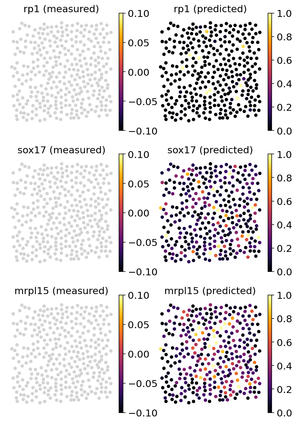
As we can see, Tangram projected the additional features onto space and we have now access to all additional genes and their estimated value at each spatial coordinate.

31.3.4. Validation on expression level

An additional step for the task of imputation might be to validate if the cell-type specific expression levels can still be recovered with the predicted counts. For this purpose, one selects a few highly expressed markers per cluster and compares the normalized expression levels. For convenience, we use the markers as described by Lu et al.[Lu et al., 2021], but one could also run a simple differential expression test between clusters to identify marker genes.

control_markers = [
    "tfrc",
    "e2f2",
    "abcb4",
    "myh10",
    "podxl",
    "cd34",
    "sdc3",
    "pzp",
    "hc",
    "mrvi1",
    "gnaz",
    "vwf",
    "kdr",
    "stab2",
    "flt4",
    "col4a1",
]

fig, ax = plt.subplots(1, len(control_markers), figsize=(25, 6.8), sharey=True)
for i, marker in enumerate(control_markers):
    # Retrieving measured counts
    measured = sc.get.obs_df(adata_st, [marker, "cell_type"])
    # Calculating measured expression levels
    measured["expression_level"] = (
        MinMaxScaler().fit(measured[[marker]]).transform(measured[[marker]])
    )

    # Retrieving measured counts
    predicted = sc.get.obs_df(ad_ge, [marker, "cell_type"])
    # Calculating predicted expression levels
    predicted["expression_level"] = (
        MinMaxScaler().fit(predicted[[marker]]).transform(predicted[[marker]])
    )

    sns.violinplot(
        data=pd.concat(
            [measured, predicted], keys=["measured", "predicted"], names=["sample"]
        ).reset_index(),
        y="cell_type",
        x="expression_level",
        hue="sample",
        split=True,
        ax=ax[i],
    )
    ax[i].set_title(marker)
    ax[i].set_xlabel("")
    ax[i].set_ylabel("")
    ax[i].get_legend().remove()
plt.tight_layout()
plt.show()

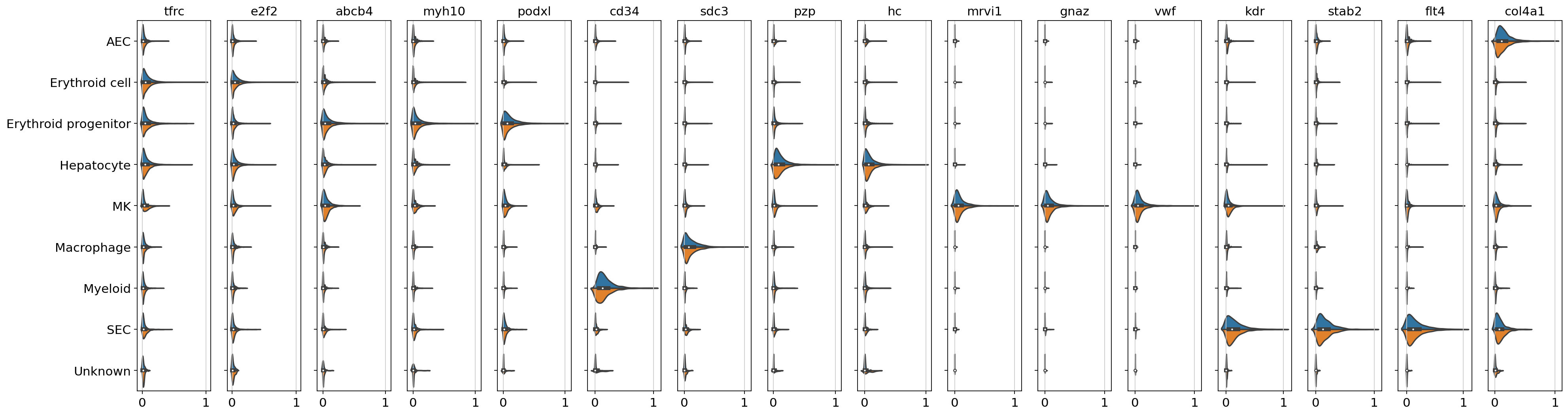
The returned plot gives us on subplot per selected marker and it’s expression level (normalized to [0,1]) for each cell type present in the dataset. As we can inspect, the cluster-wise expression levels of marker genes can still be recovered and the expression levels seem to align well within clusters. This is a good indicator that the imputation worked well and we can use the whole transcriptome spatially resolved dataset for other analysis tasks.

31.4. Key takeaways

• targeted in-situ technologies (such as MERFISH, smFISH, or seqFISH+) are limited in their gene throughput and typically only capture a few hundreds of preselected genes

• imputation methods aim to increase the resolution with respect to genes and generating whole transcriptome resolved spatially resolved data at single-cell resolution

• Tangram outperformed other imputation methods in in terms of different accuracy metrics and scalability

• Running a validation step on the shared features and their expression levels can help to assess whether the imputation algorithm worked well

31.5. References

[spatialAMMR20]

Tamim Abdelaal, Soufiane Mourragui, Ahmed Mahfouz, and Marcel J T Reinders. SpaGE: Spatial Gene Enhancement using scRNA-seq. Nucleic Acids Research, 48(18):e107–e107, 09 2020. URL: https://doi.org/10.1093/nar/gkaa740, arXiv:https://academic.oup.com/nar/article-pdf/48/18/e107/33856246/gkaa740\_supplemental\_file.pdf, doi:10.1093/nar/gkaa740.

[spatialBSB+21]

Tommaso Biancalani, Gabriele Scalia, Lorenzo Buffoni, Raghav Avasthi, Ziqing Lu, Aman Sanger, Neriman Tokcan, Charles R. Vanderburg, Åsa Segerstolpe, Meng Zhang, Inbal Avraham-Davidi, Sanja Vickovic, Mor Nitzan, Sai Ma, Ayshwarya Subramanian, Michal Lipinski, Jason Buenrostro, Nik Bear Brown, Duccio Fanelli, Xiaowei Zhuang, Evan Z. Macosko, and Aviv Regev. Deep learning and alignment of spatially resolved single-cell transcriptomes with Tangram. Nature Methods, 18(11):1352–1362, November 2021. URL: https://doi.org/10.1038/s41592-021-01264-7, doi:10.1038/s41592-021-01264-7.

[spatialLZG+22]

Bin Li, Wen Zhang, Chuang Guo, Hao Xu, Longfei Li, Minghao Fang, Yinlei Hu, Xinye Zhang, Xinfeng Yao, Meifang Tang, Ke Liu, Xuetong Zhao, Jun Lin, Linzhao Cheng, Falai Chen, Tian Xue, and Kun Qu. Benchmarking spatial and single-cell transcriptomics integration methods for transcript distribution prediction and cell type deconvolution. Nature Methods, 19(6):662–670, June 2022. URL: https://doi.org/10.1038/s41592-022-01480-9, doi:10.1038/s41592-022-01480-9.

[spatialLNL+19]

Romain Lopez, Achille Nazaret, Maxime Langevin, Jules Samaran, Jeffrey Regier, Michael I. Jordan, and Nir Yosef. A joint model of unpaired data from scrna-seq and spatial transcriptomics for imputing missing gene expression measurements. CoRR, 2019. URL: http://arxiv.org/abs/1905.02269, arXiv:1905.02269.

[spatialLLY+21] (1,2,3)

Yanfang Lu, Miao Liu, Jennifer Yang, Sherman M. Weissman, Xinghua Pan, Samuel G. Katz, and Siyuan Wang. Spatial transcriptome profiling by MERFISH reveals fetal liver hematopoietic stem cell niche architecture. Cell Discovery, 7(1):47, June 2021. URL: https://doi.org/10.1038/s41421-021-00266-1, doi:10.1038/s41421-021-00266-1.

31.6. Contributors

31.6.1. Authors

• Leon Hetzel

• Anna Schaar

31.6.2. Reviewers

• Lukas Heumos