20. Gene regulatory networks

20.1. Motivation

Once single-cell genomics data has been processed, one can dissect important relationships between observed features in their genome context. In our genome, the activation of genes is controlled in the nucleus by the RNA transcriptional machinery, which activates local (promoters) or distal cis-regulatory elements (enhancers), to control the amount of RNA produced by every gene.

Conceptually, a Gene Regulatory Network (GRN) refers to a graph representation of how certain genes that control transcription i.e. “Transcription Factors” (TF) are in charge of directly controlling the transcription rates of their target genes (cis-regulation). At the same time, such target genes once activated, can be in charge of controlling other downstream target genes (trans-regulation). Computationally, methods that infer GRNs consider the co-variation of gene and chromatin accessibility features to identify modules that could be grouped and associated simultaneously with a few TFs. A group of genes controlled by the activity of the same TF is defined as a regulon.

In addition to co-variation, several methods have recognized the gathering and injection of prior knowledge data, such as the locations where a TF bind in the genome, or previously reported TF-target gene associations, to pre-define gene-gene edges that guide the inference of GRNs that are most-supported by that type of evidence. To date, benchmarking of GRNs differs from other machine learning tasks such as image inference, in such a way that labeled data is sparse and hard to validate. For this reason, several methods have developed their own benchmark that compares new methods against others, using majorly real data. The generalization of GRN inference methods is an active discussion topic in regulatory genomics, and differently from previous chapters, requires a gold standard that is at the moment difficult to agree on and be reused consistently by the community.

The purpose of this chapter is to showcase the general pipeline of how a GRN can be generated, using methods that have been to our knowledge presented in a way that allows a validation with a low amount of software dependencies. Due to the benchmarking limitations of GRN tools in general, we recommend these tools but we cannot say that they will perform best in all possible scenarios. We would rather recommend those as a starting point, given available data, to then explore their generated GRN representations with the lowest computational effort.

20.1.1. Gathering TF regulons from public data

TF- Regulons have been annotated in academic studies, databases that compiled those, and also consortia efforts such as ENCODE. As general recommendations, one can inspect TTRUST [Han et al., 2015], DoRothEA [Garcia-Alonso et al., 2019], KnockTF [Feng et al., 2020], among others, for eukaryotic TF-regulons. For prokaryotes RegulonDB [Santos-Zavaleta et al., 2018] is a known and recognized database.

20.1.2. Limitations of TF regulons

The source and confidence of a TF-regulon have some limitations, such as data source and experimental readout. If the data source for a regulon is not matched to the cell type of interest, then results can not be put into the context of the particular biological system. Alternatively, if the experimental readout is not measuring cis regulation events, directly provoked by the TF of interest, our TF-regulon might contain trans regulation events. The usage of a TF regulon gathered in an equivalent biological system is strongly recommended. However, if those are not available the interpretation of results might be biased due to the forcing of priors.

20.1.3. Generation of GRNs using RNA data

We will explore scRNA-seq data and predicted TF-regulons, using the tool SCENIC. Specifically, we will execute SCENIC [Aibar et al., 2017] on a donor of the NeurIPS 2021 dataset, and we will interpret the results. The main processing steps described in this notebook are adapted based on SCENIC’s core tutorials Tutorial

20.1.4. Outcome of the analysis

This notebook allows interpreting single-cell RNA-seq data through the inference of a gene regulatory network, to get potential associations between Transcription Factors and target genes that explain gene expression, in contexts such as cell differentiation, transitions, and perturbations.

20.2. Dataset description

Cell-type clusters of 100,000 human PBMCs and the NeurIPS dataset, which contain healthy donors as well as COVID-19 patients[Schulte-Schrepping et al., 2020].

20.3. Environment setup

import warnings

warnings.filterwarnings("ignore")

import pyscenic
import loompy as lp
import scanpy as sc
import numpy as np
import seaborn as sns
import pandas as pd
import matplotlib.pyplot as plt
from matplotlib import rcParams
import os

20.4. Preparation of the NeurIPs dataset

The current dataset we will be looking at here is already pre-processed (previous chapters) and it contains 69,249 cells, annotated into 22 cell types. Due to batch integration considerations, we will demonstrate the usage of GRN methods for only one, labeled as s1d1 (n=6,224 cells).

Load the full dataset

adata = sc.read_h5ad("../../data/openproblems_bmmc_multiome_genes_filtered.h5ad")
adata.shape

(69249, 129921)

Subset RNA only features using the label GEX

rna = adata[:, adata.var.feature_types == "GEX"]
del adata
sc.pp.log1p(rna)
rna.obs.batch.value_counts()

s4d8     9876
s4d1     8023
s3d10    6781
s1d2     6740
s1d1     6224
s2d4     6111
s2d5     4895
s3d3     4325
s4d9     4325
s1d3     4279
s2d1     4220
s3d7     1771
s3d6     1679
Name: batch, dtype: int64

rna.shape

(69249, 13431)

Here we select highly-variable genes, to minimize the computing requirements for steps down-stream. An execution without defining HVGs is also possible, but will need additional computing memory and time.

sc.pp.highly_variable_genes(rna, batch_key="batch", flavor="seurat")

sc.set_figure_params(facecolor="white")

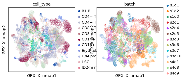
This is the embedding of all gene expression data cells of all donors. One can see that donor is dominate over cell types in terms of groups, and batch-correction methods have not been executed.

sc.pl.embedding(rna, "GEX_X_umap", color=["cell_type", "batch"])

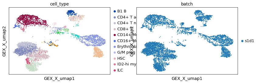
Here we observe the cells of only donor s1d1. When observing cells for only one donor, cells clusters can identified based on their provided annotations.

adata_batch = rna[rna.obs.batch == "s1d1", :]
sc.pl.embedding(adata_batch, "GEX_X_umap", color=["cell_type", "batch"])

20.5. Preparation of SCENIC

Using loompy, we will convert the gene expression values into loom files. This file format is required by pyscenic as input. In addition to this, the file allTFs_hg38.txt defines a list of gene symbols related to transcription factors, to be considered when weighting associations between those and other genes.

## this file has to be downloaded if not found
!wget -nc https://raw.githubusercontent.com/aertslab/SCENICprotocol/master/example/allTFs_hg38.txt

File ‘allTFs_hg38.txt’ already there; not retrieving.

tfs_path = "allTFs_hg38.txt"

loom_path = "data/neurips_processed_input.loom"
loom_path_output = "data/neurips_processed_output.loom"
tfs = [tf.strip() for tf in open(tfs_path)]

As a verification, it is recommended to check that genes annotated as TFs are part of the provided input data. If not a high coverage of gene symbols is observed e.g. 50% or more, there could be an issues with the feature names declared in the .var, such as Ensembl IDs instead of gene_symbols, or lower/uppercase difference if the genome assembly is mouse or another species that uses a different capitalization style than human.

# as a general QC. We inspect that our object has transcription factors listed in our main annotations.
print(
    f"%{np.sum(adata_batch.var.index.isin(tfs))} out of {len(tfs)} TFs are found in the object"
)

1160 out of 1797 TFs are found in the object

Usage of HVG or all features can be defined here, by changing the flag use_hvg to False.

use_hvg = True
if use_hvg:
    mask = (adata_batch.var["highly_variable"] == True) | adata_batch.var.index.isin(
        tfs
    )
    adata_batch = adata_batch[:, mask]

Create a loom file for NeurIPS donor. If you get an error in this step, verify that the labels for Gene/CellID/etc. are properly defined.

row_attributes = {
    "Gene": np.array(adata_batch.var.index),
}
col_attributes = {
    "CellID": np.array(adata_batch.obs.index),
    "nGene": np.array(np.sum(adata_batch.X.transpose() > 0, axis=0)).flatten(),
    "nUMI": np.array(np.sum(adata_batch.X.transpose(), axis=0)).flatten(),
}

lp.create(loom_path, adata_batch.X.transpose(), row_attributes, col_attributes)

Once the loom file has been generated, we execute pyscenic to generate associations between TFs and genes. TF-gene associations are inferred by GRNBoost, and summarized by a directional weight between TFs and target genes. The output of this analysis is a table summarizing all reported associations with their importance weight.

Some steps below require indicating a number of cores (num_workers). Increase according to computing resources available

num_workers = 3

outpath_adj = "adj.csv"
if not os.path.exists(outpath_adj):
    !pyscenic grn {loom_path} {tfs_path} -o $outpath_adj --num_workers {num_workers}

Show the top of TF-target associations

results_adjacencies = pd.read_csv("adj.csv", index_col=False, sep=",")
print(f"Number of associations: {results_adjacencies.shape[0]}")
results_adjacencies.head()

# associations: 683484

	TF	target	importance
0	SOX6	SLC4A1	186.835278
1	SOX6	ANK1	162.917264
2	SOX6	HBA2	143.750583
3	SOX6	SLC25A37	127.603415
4	HMGB2	UBE2S	123.732197

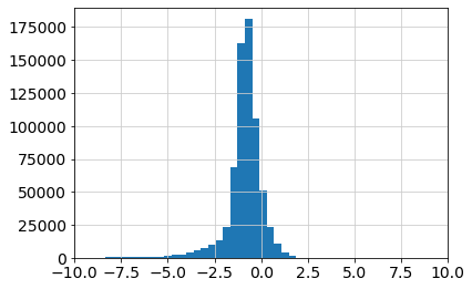
Visualize the distribution of weights for general inspection of the quantiles and thresholds obtained from pyscenic. As provided by the pyscenic grn step, the importance scores follow a unimodal distribution, with negative/positive values indicating TF-gene associations with less/more importance, respectively. From the right-tail of this distribution, we can recover the most relevant interactions between TFs and potential target genes, supported by gene expression values and the analysis done by pyscenic.

plt.hist(np.log10(results_adjacencies["importance"]), bins=50)
plt.xlim([-10, 10])

(-10.0, 10.0)

As targets genes have DNA motifs at promoters (sequence specific DNA motifs), those can be used to link TFs to target genes. Next, we use an annotation of TF associations to Transcription Start Sites (TSSs) to refine this annotation.

Download TSS annotations precalculated by Aerts’s lab

!wget -nc https://resources.aertslab.org/cistarget/databases/homo_sapiens/hg38/refseq_r80/mc9nr/gene_based/hg38__refseq-r80__10kb_up_and_down_tss.mc9nr.genes_vs_motifs.rankings.feather

File ‘hg38__refseq-r80__10kb_up_and_down_tss.mc9nr.genes_vs_motifs.rankings.feather’ already there; not retrieving.

import glob
import os

# ranking databases
db_glob = "*feather"
db_names = " ".join(glob.glob(db_glob))

Download a catalog of motif-to-TF associations

!wget -nc https://resources.aertslab.org/cistarget/motif2tf/motifs-v9-nr.hgnc-m0.001-o0.0.tbl

File ‘motifs-v9-nr.hgnc-m0.001-o0.0.tbl’ already there; not retrieving.

# motif databases
motif_path = "motifs-v9-nr.hgnc-m0.001-o0.0.tbl"

Using the catalog of motif and their gene associations at promoters, retrieved a subset adjacencies by pruning of the previous adjacencies. This step can take several minutes on consumer grade hardware.

if not os.path.exists('reg.csv'):
    !pyscenic ctx adj.csv \
        {db_names} \
        --annotations_fname {motif_path} \
        --expression_mtx_fname {loom_path} \
        --output reg.csv \
        --mask_dropouts \
        --num_workers {num_workers} > pyscenic_ctx_stdout.txt

To explore the candidates reported, it is recommended as a rule of thumb to explore the output by the ranking of relative contribution, or by top-quantile thresholds defined visually to obtain a high signal-to-noise ratio.

Define custom quantiles for further exploration

import numpy as np

n_genes_detected_per_cell = np.sum(adata_batch.X > 0, axis=1)
percentiles = pd.Series(n_genes_detected_per_cell.flatten().A.flatten()).quantile(
    [0.01, 0.05, 0.10, 0.50, 1]
)
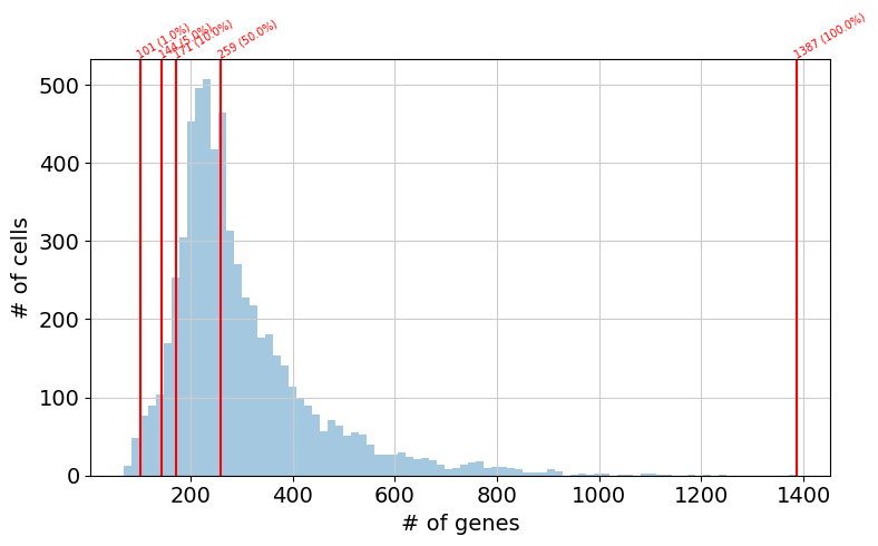
print(percentiles)

0.01     101.0
0.05     144.0
0.10     171.0
0.50     259.0
1.00    1387.0
dtype: float64

The histogram below indicates the distribution of genes detected per cell. This visualization is convenient to define the parameter --auc_threshold in the next step. Specifically, the default parameter of --auc_threshold is 0.05, which in this plot would result in the selection of 144 genes, to be used as a reference per cell for AUCell calculations. The modification of this parameter affects the estimation of AUC values calculated by AUCell.

fig, ax = plt.subplots(1, 1, figsize=(8, 5), dpi=100)
sns.distplot(n_genes_detected_per_cell, norm_hist=False, kde=False, bins="fd")
for i, x in enumerate(percentiles):
    fig.gca().axvline(x=x, ymin=0, ymax=1, color="red")
    ax.text(
        x=x,
        y=ax.get_ylim()[1],
        s=f"{int(x)} ({percentiles.index.values[i]*100}%)",
        color="red",
        rotation=30,
        size="x-small",
        rotation_mode="anchor",
    )
ax.set_xlabel("# of genes")
ax.set_ylabel("# of cells")
fig.tight_layout()

This step will use TFs to calculate Area Under the Curve scores, that summarize how well the gene expression observed in each cell can be associated by the regulation of target genes regulatred by the mentioned TFs.

Using the above-generated matrix of cell x TFs and those scores, we can calculate a new embedding using only those.

if not os.path.exists(loom_path_output):
    !pyscenic aucell $loom_path \
        reg.csv \
        --output {loom_path_output} \
        --num_workers {num_workers} > pyscenic_aucell_stdout.txt

import json
import zlib
import base64

# collect SCENIC AUCell output
lf = lp.connect(loom_path_output, mode="r+", validate=False)
auc_mtx = pd.DataFrame(lf.ca.RegulonsAUC, index=lf.ca.CellID)
lf.close()

import anndata as ad

ad_auc_mtx = ad.AnnData(auc_mtx)
sc.pp.neighbors(ad_auc_mtx, n_neighbors=10, metric="correlation")
sc.tl.umap(ad_auc_mtx)
sc.tl.tsne(ad_auc_mtx)

WARNING: You’re trying to run this on 247 dimensions of `.X`, if you really want this, set `use_rep='X'`.
         Falling back to preprocessing with `sc.pp.pca` and default params.

Visualize the data base on the TF-regulons and auc_mtx generated.

adata_batch.obsm["X_umap_aucell"] = ad_auc_mtx.obsm["X_umap"]
adata_batch.obsm["X_tsne_aucell"] = ad_auc_mtx.obsm["X_tsne"]

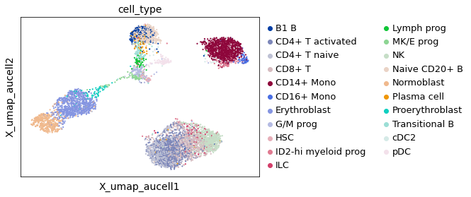
This UMAP visualization confirms that the signal from SCENIC is capable of capturing regulons that keep dividing most cell populations into sub-groups. Hence, there is information TF-regulons that enables cell-type identification.

sc.pl.embedding(adata_batch, basis="X_umap_aucell", color="cell_type")

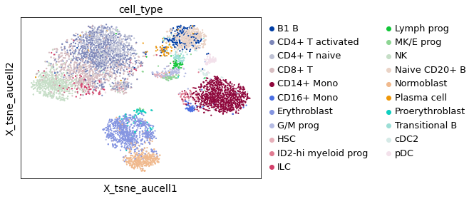
A visualization of the tSNE values generated by SCENIC also confimrs this cell-type separation, for the majority of cell-types

sc.pl.embedding(adata_batch, basis="X_tsne_aucell", color="cell_type")

20.5.1. Interpretation of results

import seaborn as sns

auc_mtx["cell_type"] = adata_batch.obs["cell_type"]
mean_auc_by_cell_type = auc_mtx.groupby("cell_type").mean()

show the top N TF regulons by a color

top_n = 50
top_tfs = mean_auc_by_cell_type.max(axis=0).sort_values(ascending=False).head(top_n)
mean_auc_by_cell_type_top_n = mean_auc_by_cell_type[
    [c for c in mean_auc_by_cell_type.columns if c in top_tfs]
]

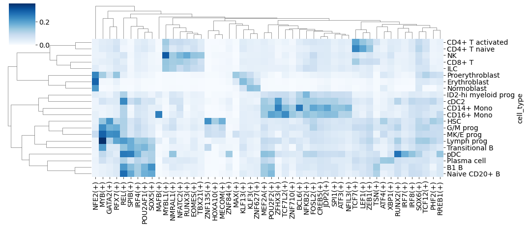
Once we know the top TF-regulons involved in the biological system we are studying, we can inspect the activities estimated by each TF, based on the scores per cell, or the overall AUCs per cell-type explained by those TF (blue heatmap below).

sns.clustermap(
    mean_auc_by_cell_type_top_n,
    figsize=[15, 6.5],
    cmap="Blues",
    xticklabels=True,
    yticklabels=True,
)

<seaborn.matrix.ClusterGrid at 0x7fc377ccce10>

As the red heatmap is suggesting that some TFs are strongly associated to particular cell types, we can verify the expression of their expression levels as an additional validation. This is done by matching the TF names we want to highlight, and visualize those using Scanpy’s (red heatmap).

tf_names = top_tfs.index.str.replace("\(\+\)", "")
adata_batch_top_tfs = adata_batch[:, adata_batch.var_names.isin(tf_names)]

sc.pl.matrixplot(
    adata_batch,
    tf_names,
    groupby="cell_type",
    cmap="Reds",
    dendrogram=True,
    figsize=[15, 5.5],
    standard_scale="group",
)

WARNING: dendrogram data not found (using key=dendrogram_cell_type). Running `sc.tl.dendrogram` with default parameters. For fine tuning it is recommended to run `sc.tl.dendrogram` independently.
WARNING: You’re trying to run this on 2785 dimensions of `.X`, if you really want this, set `use_rep='X'`.
         Falling back to preprocessing with `sc.pp.pca` and default params.

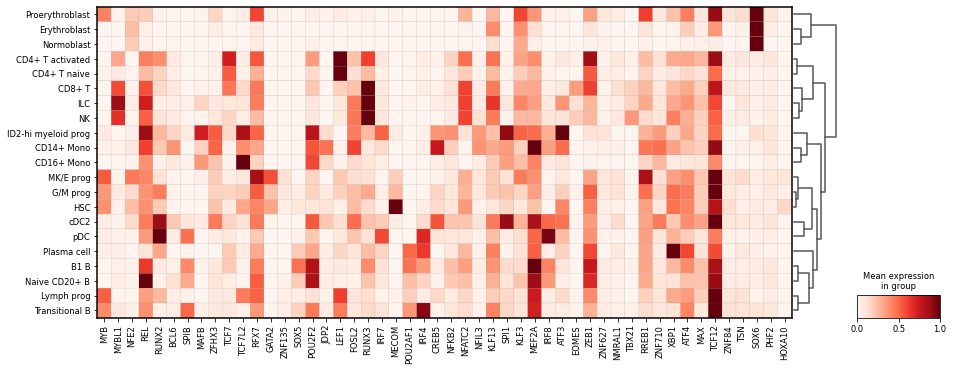
Through visual inspection and comparison of the TF-regulon AUC scores and TF gene expression by cell type, we can verify that in several case the cell-type specific expression of a TF is linked to a particular cell type, where the respective TF-regulon is also active e.g. RUNX2 in pDCs, TCF7L2 in CD16+ Mono, LEF1 in CD4+ T activated. Additional inspection can serve to validate previous insights and/or additional associations.

20.6. Takeaways

In this notebook, we have:

1. Setup a basic pipeline to prepare, execute, and verify SCENIC results using the NeurIPs 2021 dataset.

2. Detected TF-regulons that allow to explain the observed transcriptomes by the regulatory potential of a handful of TFs.

20.7. Quiz

20.7.1. Theory

1. How many genes in the human/mouse genome are considered TFs?

2. What is a TF-regulon?

3. How many DNA-binding motifs are there to each TFs? 3.1. Currently, are there more known DNA-binding motifs or TFs that bind those? 3.2. How can one reconcile the redundancy of these during the analysis?

4. Additional reading: Describe the futility theorem.

20.7.2. SCENIC

1. Describe the major steps in the SCENIC pipeline (three or more)?

2. What could happen if the number of TFs reported in your own data has a low overlap to the one externally retrieved?

3. What is the AUC score from pyscenic and how it can be helpful for interpretation of results per cell cluster?

20.8. References

[grnAGonzalezBM+17]

Sara Aibar, Carmen Bravo González-Blas, Thomas Moerman, Vân Anh Huynh-Thu, Hana Imrichova, Gert Hulselmans, Florian Rambow, Jean-Christophe Marine, Pierre Geurts, Jan Aerts, Joost van den Oord, Zeynep Kalender Atak, Jasper Wouters, and Stein Aerts. SCENIC: single-cell regulatory network inference and clustering. Nat. Methods, 14(11):1083–1086, November 2017.

[grnFSL+20]

Chenchen Feng, Chao Song, Yuejuan Liu, Fengcui Qian, Yu Gao, Ziyu Ning, Qiuyu Wang, Yong Jiang, Yanyu Li, Meng Li, Jiaxin Chen, Jian Zhang, and Chunquan Li. KnockTF: a comprehensive human gene expression profile database with knockdown/knockout of transcription factors. Nucleic Acids Res., 48(D1):D93–D100, January 2020.

[grnGAHI+19]

Luz Garcia-Alonso, Christian H Holland, Mahmoud M Ibrahim, Denes Turei, and Julio Saez-Rodriguez. Benchmark and integration of resources for the estimation of human transcription factor activities. Genome Res., 29(8):1363–1375, August 2019.

[grnHSS+15]

Heonjong Han, Hongseok Shim, Donghyun Shin, Jung Eun Shim, Yunhee Ko, Junha Shin, Hanhae Kim, Ara Cho, Eiru Kim, Tak Lee, Hyojin Kim, Kyungsoo Kim, Sunmo Yang, Dasom Bae, Ayoung Yun, Sunphil Kim, Chan Yeong Kim, Hyeon Jin Cho, Byunghee Kang, Susie Shin, and Insuk Lee. TRRUST: a reference database of human transcriptional regulatory interactions. Sci. Rep., 5:11432, June 2015.

[grnSZSanchezPerezS+18]

Alberto Santos-Zavaleta, Mishael Sánchez-Pérez, Heladia Salgado, David A Velázquez-Ramírez, Socorro Gama-Castro, Víctor H Tierrafría, Stephen J W Busby, Patricia Aquino, Xin Fang, Bernhard O Palsson, James E Galagan, and Julio Collado-Vides. A unified resource for transcriptional regulation in escherichia coli K-12 incorporating high-throughput-generated binding data into RegulonDB version 10.0. BMC Biol., 16(1):91, August 2018.

[grnSSRP+20]

Jonas Schulte-Schrepping, Nico Reusch, Daniela Paclik, Kevin Baßler, Stephan Schlickeiser, Bowen Zhang, Benjamin Krämer, Tobias Krammer, Sophia Brumhard, Lorenzo Bonaguro, Elena De Domenico, Daniel Wendisch, Martin Grasshoff, Theodore S. Kapellos, Michael Beckstette, Tal Pecht, Adem Saglam, Oliver Dietrich, Henrik E. Mei, Axel R. Schulz, Claudia Conrad, Désirée Kunkel, Ehsan Vafadarnejad, Cheng-Jian Xu, Arik Horne, Miriam Herbert, Anna Drews, Charlotte Thibeault, Moritz Pfeiffer, Stefan Hippenstiel, Andreas Hocke, Holger Müller-Redetzky, Katrin-Moira Heim, Felix Machleidt, Alexander Uhrig, Laure Bosquillon de Jarcy, Linda Jürgens, Miriam Stegemann, Christoph R. Glösenkamp, Hans-Dieter Volk, Christine Goffinet, Markus Landthaler, Emanuel Wyler, Philipp Georg, Maria Schneider, Chantip Dang-Heine, Nick Neuwinger, Kai Kappert, Rudolf Tauber, Victor Corman, Jan Raabe, Kim Melanie Kaiser, Michael To Vinh, Gereon Rieke, Christian Meisel, Thomas Ulas, Matthias Becker, Robert Geffers, Martin Witzenrath, Christian Drosten, Norbert Suttorp, Christof von Kalle, Florian Kurth, Kristian Händler, Joachim L. Schultze, Anna C. Aschenbrenner, Yang Li, Jacob Nattermann, Birgit Sawitzki, Antoine-Emmanuel Saliba, Leif Erik Sander, and Deutsche COVID-19 OMICS Initiative (DeCOI). Severe covid-19 is marked by a dysregulated myeloid cell compartment. Cell, 182(6):1419–1440.e23, Sep 2020. S0092-8674(20)30992-2[PII]. URL: https://doi.org/10.1016/j.cell.2020.08.001, doi:10.1016/j.cell.2020.08.001.

20.9. Contributors

We gratefully acknowledge the contributions of:

20.9.1. Authors

• Ignacio Ibarra

20.9.2. Reviewers

• Lukas Heumos

• Anna Schaar