12. Clustering#
Key takeaways
Use Leiden community detection on a single-cell KNN graph.
Sub-clustering with different resolution parameters allows the user to focus on more detailed substructures in the dataset to potentially identify finer cell states.
Environment setup
Install conda:
Before creating the environment, ensure that conda is installed on your system.
Save the yml content:
Copy the content from the yml tab into a file named
environment.yml.
Create the environment:
Open a terminal or command prompt.
Run the following command:
conda env create -f environment.yml
Activate the environment:
After the environment is created, activate it using:
conda activate <environment_name>
Replace
<environment_name>with the name specified in theenvironment.ymlfile. In the yml file it will look like this:name: <environment_name>
Verify the installation:
Check that the environment was created successfully by running:
conda env list
name: clustering
channels:
  - defaults
  - conda-forge
dependencies:
  - conda-forge::python=3.13
  - conda-forge::scanpy=1.11.5
  - conda-forge::pynndescent=0.5.13
  - conda-forge::ipykernel=7.1.0
  - pip
  - pip:
      - igraph==1.0.0
      - lamindb
Get data and notebooks
This book uses lamindb to store, share, and load datasets and notebooks using the theislab/sc-best-practices instance. We acknowledge free hosting from Lamin Labs.
Install lamindb
Install the lamindb Python package:
pip install lamindb
Optionally create a lamin account
Sign up and log in following the instructions
Verify your setup
Run the
lamin connectcommand:
import lamindb as ln

ln.Artifact.connect("theislab/sc-best-practices").df()
You should now see up to 100 of the stored datasets.
Accessing datasets (Artifacts)
Search for the datasets on the Artifacts page
Load an Artifact and the corresponding object:
import lamindb as ln
af = ln.Artifact.connect("theislab/sc-best-practices").get(key="key_of_dataset", is_latest=True)
obj = af.load()
The object is now accessible in memory and is ready for analysis. Adapt the
lamindb.Artifact.connect("theislab/sc-best-practices").get("SOMEIDXXXX")suffix to get respective versions.Accessing notebooks (Transforms)
Search for the notebook on the Transforms page
Load the notebook:
lamin load <notebook url>
which will download the notebook to the current working directory. Analogously to
Artifacts, you can adapt the suffix ID to get older versions.
12.1. Motivation#
Preprocessing and visualization enabled us to describe our scRNA-seq dataset and reduce its dimensionality. Up to this point, we embedded and visualized cells to understand the underlying properties of our dataset. However, they are still rather abstractly defined. The next natural step in single-cell analysis is the identification of cellular structure in the dataset.
In scRNA-seq data analysis, we describe cellular structure in our dataset by finding cell identities that relate to known cell states or cell cycle stages. This process is usually called cell identity annotation. For this purpose, we structure cells into clusters to infer the identity of similar cells. Clustering itself is a common unsupervised machine learning problem. We can derive clusters by minimizing the intra-cluster distance in the reduced expression space. In this case, the expression space determines the gene expression similarity of cells with respect to a dimensionality-reduced representation. This lower-dimensional representation is, for example, determined with a principal-component analysis, and the similarity scoring is then based on Euclidean distances.
The KNN(K-Nearest-Neighbor) graph consists of nodes reflecting the cells in the dataset.
We first calculate a Euclidean distance matrix on the PC-reduced expression space for all cells and then connect each cell to its K most similar cells.
Usually, K is set to values between 5 and 100, depending on the size of the dataset.
The KNN graph reflects the underlying topology of the expression data by representing dense regions with respect to expression space, as well as as densely connected regions in the graph [Wolf et al., 2019].
Dense regions in the KNN-graph are detected by community detection methods like Leiden and Louvain[Blondel et al., 2008].
PC-reduced expression space
PC-reduced expression space refers to the lower-dimensional space obtained after using Principal Component Analysis (PCA) to high-dimensional gene expression data. After PCA, for example, we are working with the top 10-50 principal components instead of 20,000 genes.
The Leiden algorithm is an improved version of the Louvain algorithm, which outperformed other clustering methods for single-cell RNA-seq data analysis ([Du et al., 2018, Freytag et al., 2018, Weber and Robinson, 2016]). Since the Louvain algorithm is no longer maintained, using Leiden instead is preferred.
We, therefore, propose to use the Leiden algorithm[Traag et al., 2019] on single-cell k-nearest-neighbour (KNN) graphs to cluster single-cell datasets.
Leiden creates clusters by taking into account the number of links between cells in a cluster versus the overall expected number of links in the dataset.
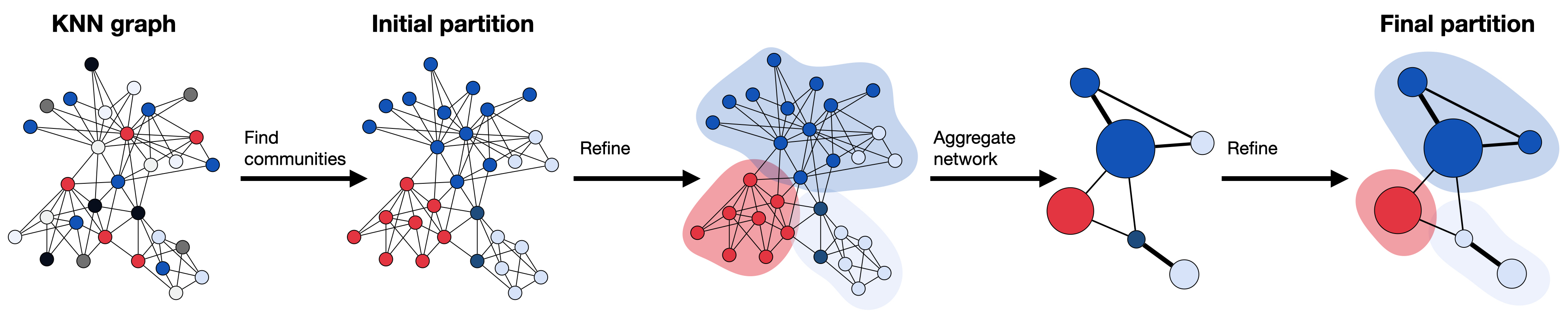
Fig. 12.1 The Leiden algorithm computes a clustering on a KNN graph obtained from the PC reduced expression space. The starting point is a singleton partition in which each node functions as its own community. As a next step, the algorithm creates partitions by moving individual nodes from one community to another, which is refined afterwards to enhance the partitioning. The refined partition is then aggregated to a network. Subsequently, the algorithm moves again individual nodes in the aggregate network, until refinement no longer changes the partition. All steps are repeated until the final clustering is created and partitions no longer change.#
The Leiden module has a resolution parameter that allows for determining the scale of the partition cluster and therefore the coarseness of the clustering. A higher resolution parameter leads to more clusters. The algorithm additionally allows efficient sub-clustering of particular clusters in the dataset by sub-setting the KNN graph. Sub-clustering enables the user to identify cell-type specific states within clusters or a finer cell type labeling[Wagner et al., 2016], but can also lead to patterns that are only due to noise present in the data.
As mentioned before, the Leiden algorithm is implemented in scanpy.
Running this on a GPU
Leiden clustering on a million-cell graph is one of the worst CPU bottlenecks in a typical pipeline and one of the best GPU wins.
rapids-singlecell provides rapids_singlecell.tl.leiden() with the same signature and routinely runs 50–100× faster than the CPU implementation.
import lamindb as ln
import scanpy as sc

assert ln.setup.settings.instance.slug == "theislab/sc-best-practices"

ln.track("rJhR7SskiROg")

# Configuring scanpy's settings for outfits and visualization
sc.settings.verbosity = 0
sc.settings.set_figure_params(dpi=80, facecolor="white", frameon=False)
→ loaded Transform('rJhR7SskiROg0000', key='clustering.ipynb'), re-started Run('LZOdfrBECJI7FQWH4MFl') at 2026-02-16 13:15:47 UTC
→ notebook imports: lamindb==2.0.1 scanpy==1.11.5
12.2. Clustering human bone marrow cells#
Firstly, we load our dataset.
We perform clustering on the preprocessed sample site4-donor8 from the NeurIPS human bone marrow dataset, which we already preprocessed and uploaded to our LaminDB.
This dataset was normalized with scran.
af = ln.Artifact.get(key="cellular_structure/s4d8_subset.h5ad", is_latest=True)
adata = af.load()
The Leiden algorithm leverages a KNN graph on the reduced expression space.
We can calculate the KNN graph on a lower-dimensional gene expression representation with the scanpy function scanpy.pp.neighbors().
We call this function on the top 30 principal-components as these capture most of the variance in the dataset.
Visualizing the clustering can help us to understand the results, we therefore embed our cells into a UMAP embedding.
More details can be found in the dimensionality reduction chapter.
sc.pp.neighbors(adata, n_pcs=30)
sc.tl.umap(adata)
We can now call the Leiden algorithm.
sc.tl.leiden(adata, flavor="igraph", n_iterations=2)
Optimizing Leiden Iterations
The n_iterations parameter in scanpy.tl.leiden() determines how many refinement passes the algorithm performs to optimize its community detection.
n_iterations = 2(Recommended): The standard choice for most analyses. It offers a significant boost in cluster quality over the Louvain algorithm while remaining computationally efficient.n_iterations = -1(Optimal): Forces the algorithm to run until it reaches full convergence. While this produces the “perfect” mathematical clustering, it can be significantly slower on large datasets.n_iterations > 2: Allows you to specify a fixed number of passes to balance precision and speed.
Tip: Even at 2 iterations, Leiden effectively prevents the “disconnected clusters” issue often found in older methods.
In scanpy, the resolution parameter is used in clustering methods, such as the Louvain or Leiden methods. It controls the granularity or coarseness of the resulting clusters. The default resolution parameter in scanpy is 1.0. However, in many cases the analyst may want to try different resolution parameters to control the coarseness of the clustering. Hence, we recommend to save the clustering result under a specified key which indicates the selected resolution.
sc.tl.leiden(
    adata, key_added="leiden_res0_25", resolution=0.25, flavor="igraph", n_iterations=2
)
sc.tl.leiden(
    adata, key_added="leiden_res0_5", resolution=0.5, flavor="igraph", n_iterations=2
)
sc.tl.leiden(
    adata, key_added="leiden_res1", resolution=1.0, flavor="igraph", n_iterations=2
)
We now visualize the different clustering results obtained with the Leiden algorithm at different resolutions. As we can see, the resolution heavily influences how coarse our clustering is. Higher resolution parameters lead to more communities, i.e., more identified clusters, while lower resolution parameters lead to fewer communities. You can think of it like zooming, where we take a closer look at the clusters with higher resolution. The resolution parameter, therefore, controls how densely clustered regions in the KNN-embedding are grouped together by the algorithm. This will become especially important for annotating the clusters.
sc.pl.umap(
    adata,
    color=["leiden_res0_25", "leiden_res0_5", "leiden_res1"],
    legend_loc="on data",
)
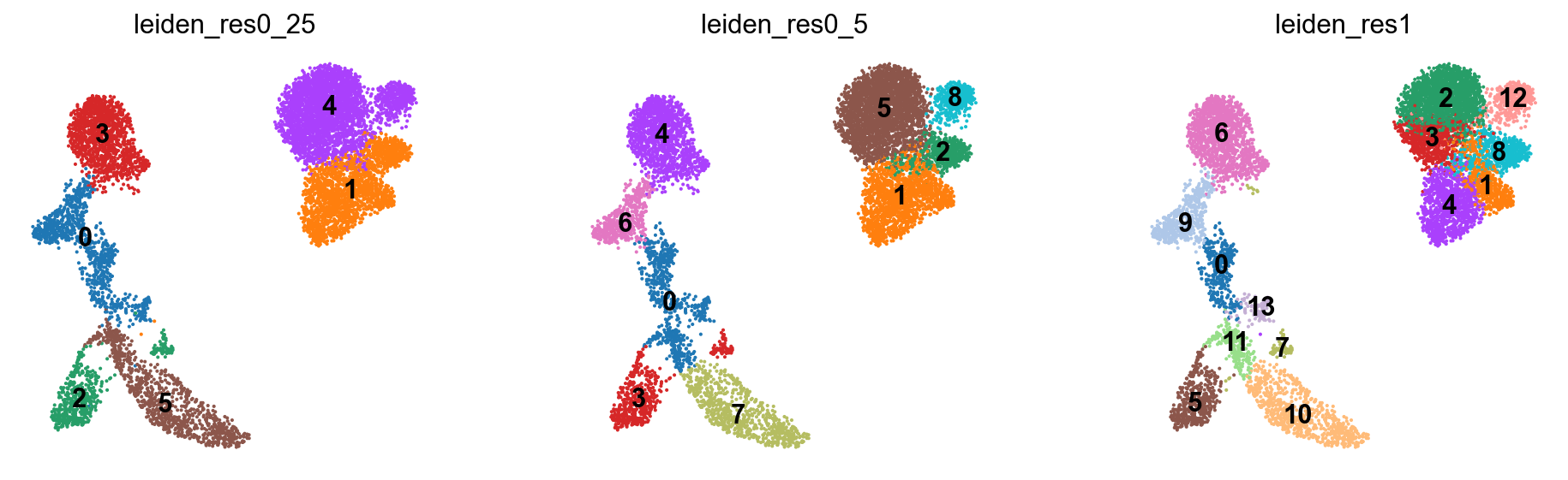
We now clearly inspect the impact of different resolutions on the clustering result. For a resolution of 0.25, the clustering is much coarser, and the algorithm detected fewer communities. Additionally, clustered regions are less dense compared to the clustering obtained at a resolution of 1.0.
We would like to highlight again that distances between the displayed clusters must be interpreted with caution. As the UMAP embedding is in 2D, distances are not necessarily captured well between all points. We recommend not interpreting distances between clusters visualized on UMAP embeddings.
As usual, we will upload the processed anndata to lamindb.
You can skip this part.
af = ln.Artifact.from_anndata(
    adata,
    key="cellular_structure/s4d8_clustered.h5ad",
    description="anndata after clustering",
).save()
af
→ writing the in-memory object into cache
→ returning artifact with same hash: Artifact(uid='UIb3nBOY3Xcejedh0003', version_tag=None, is_latest=True, key='cellular_structure/s4d8_clustered.h5ad', description='anndata after clustering', suffix='.h5ad', kind='dataset', otype='AnnData', size=364819346, hash='20SV0Ax1_Ot0qHUM0DgM9Q', n_files=None, n_observations=8874, branch_id=1, space_id=1, storage_id=1, run_id=11, schema_id=None, created_by_id=5, created_at=2026-02-16 14:57:06 UTC, is_locked=False); to track this artifact as an input, use: ln.Artifact.get()
Artifact(uid='UIb3nBOY3Xcejedh0003', version_tag=None, is_latest=True, key='cellular_structure/s4d8_clustered.h5ad', description='anndata after clustering', suffix='.h5ad', kind='dataset', otype='AnnData', size=364819346, hash='20SV0Ax1_Ot0qHUM0DgM9Q', n_files=None, n_observations=8874, branch_id=1, space_id=1, storage_id=1, run_id=11, schema_id=None, created_by_id=5, created_at=2026-02-16 14:57:06 UTC, is_locked=False)
12.3. References#
Vincent D. Blondel, Jean-Loup Guillaume, Renaud Lambiotte, and Etienne Lefebvre. Fast unfolding of communities in large networks. Journal of Statistical Mechanics: Theory and Experiment, 2008(10):P10008, October 2008. Publisher: IOP Publishing. URL: https://doi.org/10.1088/1742-5468/2008/10/p10008, doi:10.1088/1742-5468/2008/10/p10008.
A Du, MD Robinson, and C Soneson. A systematic performance evaluation of clustering methods for single-cell term`RNA`-seq data [version 1; peer review: 2 approved with reservations]. F1000Research, 2018. doi:10.12688/f1000research.15666.1.
S Freytag, L Tian, I L�nnstedt, M Ng, and M Bahlo. Comparison of clustering tools in R for medium-sized 10x Genomics single-cell term`RNA`-sequencing data [version 1; peer review: 1 approved, 2 approved with reservations]. F1000Research, 2018. doi:10.12688/f1000research.15809.1.
V. A. Traag, L. Waltman, and N. J. van Eck. From Louvain to Leiden: guaranteeing well-connected communities. Scientific Reports, 9(1):5233, March 2019. URL: https://doi.org/10.1038/s41598-019-41695-z, doi:10.1038/s41598-019-41695-z.
Allon Wagner, Aviv Regev, and Nir Yosef. Revealing the vectors of cellular identity with single-cell genomics. Nature Biotechnology, 34(11):1145–1160, November 2016. URL: https://doi.org/10.1038/nbt.3711, doi:10.1038/nbt.3711.
Lukas M. Weber and Mark D. Robinson. Comparison of clustering methods for high-dimensional single-cell flow and mass cytometry data. Cytometry Part A, 89(12):1084–1096, 2016. _eprint: https://onlinelibrary.wiley.com/doi/pdf/10.1002/cyto.a.23030. URL: https://onlinelibrary.wiley.com/doi/abs/10.1002/cyto.a.23030, doi:https://doi.org/10.1002/cyto.a.23030.
F. Alexander Wolf, Fiona K. Hamey, Mireya Plass, Jordi Solana, Joakim S. Dahlin, Berthold Göttgens, Nikolaus Rajewsky, Lukas Simon, and Fabian J. Theis. PAGA: graph abstraction reconciles clustering with trajectory inference through a topology preserving map of single cells. Genome Biology, 20(1):59, March 2019. URL: https://doi.org/10.1186/s13059-019-1663-x, doi:10.1186/s13059-019-1663-x.
12.4. Contributors#
We gratefully acknowledge the contributions of:
12.4.2. Reviewers#
Lukas Heumos