38. Batch correction#
Key takeaways
Due to pronounced batch effects in ADT data, methods like Harmony, originally designed for transcriptomics data, are recommended for batch correction, as they effectively integrate samples and maintain cell type separation.
Environment setup
Install conda:
Before creating the environment, ensure that conda is installed on your system.
Save the yml content:
Copy the content from the yml tab into a file named
environment.yml.
Create the environment:
Open a terminal or command prompt.
Run the following command:
conda env create -f environment.yml
Activate the environment:
After the environment is created, activate it using:
conda activate <environment_name>
Replace
<environment_name>with the name specified in theenvironment.ymlfile. In the yml file it will look like this:name: <environment_name>
Verify the installation:
Check that the environment was created successfully by running:
conda env list
name: surface-protein
channels:
  - conda-forge
dependencies:
  - python=3.13
  - scanpy=1.12
  - muon=0.1.7
  - python-igraph=1.0.0
  - ipykernel=7.2.0
  - pip==26.0.1
  - pip:
      - lamindb==2.3.1
      - harmonypy==0.0.9
Get data and notebooks
This book uses lamindb to store, share, and load datasets and notebooks using the theislab/sc-best-practices instance. We acknowledge free hosting from Lamin Labs.
Install lamindb
Install the lamindb Python package:
pip install lamindb
Optionally create a lamin account
Sign up and log in following the instructions
Verify your setup
Run the
lamin connectcommand:
import lamindb as ln

ln.Artifact.connect("theislab/sc-best-practices").df()
You should now see up to 100 of the stored datasets.
Accessing datasets (Artifacts)
Search for the datasets on the Artifacts page
Load an Artifact and the corresponding object:
import lamindb as ln
af = ln.Artifact.connect("theislab/sc-best-practices").get(key="key_of_dataset", is_latest=True)
obj = af.load()
The object is now accessible in memory and is ready for analysis. Adapt the
lamindb.Artifact.connect("theislab/sc-best-practices").get("SOMEIDXXXX")suffix to get respective versions.Accessing notebooks (Transforms)
Search for the notebook on the Transforms page
Load the notebook:
lamin load <notebook url>
which will download the notebook to the current working directory. Analogously to
Artifacts, you can adapt the suffix ID to get older versions.
38.1. Motivation#
As could be seen for our earlier visualized ADT data, batch effects between donors are very pronounced (see Dimensionality Reduction). Hence, batch correction to mitigate this effect is required.
We use Harmony here. There is no benchmarking of different batch correction methods for ADT data. We therefore use Harmony, a method that has been benchmarked for scRNA-seq data with good results.
Recently two batch correction methods for ADT data have been published in reputable journals and/or by reputable authors: ADTnorm [Zheng et al., 2025] and CytoVI [Ingelfinger et al., 2025]. These two methods might be appropriate for ADT data. However, as mentioned, here we stick to Harmony, which is more proven and independently benchmarked (although for transcriptomics and not for ADT data).
38.2. Environment setup#
import warnings

import muon as mu
import scanpy as sc

warnings.filterwarnings("ignore")
mu.set_options(pull_on_update=False)
sc.settings.verbosity = 0
sc.set_figure_params(
    dpi=80,
    facecolor="white",
    frameon=False,
)

import lamindb as ln

ln.track()
→ found notebook batch_correction.ipynb, making new version
→ created Transform('4LJehi0GPRuj0003', key='batch_correction.ipynb'), started new Run('9GLRcMWow8KIOWYb') at 2026-04-10 17:31:12 UTC
→ notebook imports: lamindb-core==2.3.1 muon==0.1.7 scanpy==1.12
• recommendation: to identify the notebook across renames, pass the uid: ln.track("4LJehi0GPRuj")
38.3. Loading the data#
We load the MuData object we saved at the end of the previous chapter Dimensionality Reduction:
af = ln.Artifact.connect("theislab/sc-best-practices").get(
    key="surface-protein/cite_dimensionality_reduction.h5mu", is_latest=True
)
mdata = af.load()
mdata
MuData object with n_obs × n_vars = 117951 × 36737
  var:	'gene_ids', 'feature_types'
  2 modalities
    rna:	117951 x 36601
      obs:	'donor', 'batch'
      var:	'gene_ids', 'feature_types'
    prot:	117951 x 136
      obs:	'donor', 'batch', 'n_genes_by_counts', 'log1p_n_genes_by_counts', 'total_counts', 'log1p_total_counts', 'n_counts', 'outliers', 'doublets_markers'
      var:	'gene_ids', 'feature_types', 'n_cells_by_counts', 'mean_counts', 'log1p_mean_counts', 'pct_dropout_by_counts', 'total_counts', 'log1p_total_counts'
      uns:	'batch_colors', 'donor_colors', 'doublets_markers_colors', 'neighbors', 'pca', 'umap'
      obsm:	'X_pca', 'X_umap'
      varm:	'PCs'
      obsp:	'connectivities', 'distances'
38.4. Harmony#
It is not yet clear which batch effect correction works best for ADT data. For general purposes we recommend Harmony [Korsunsky et al., 2019] to perform batch correction of the data due to its robust performance on scRNA-seq data.
sc.external.pp.harmony_integrate(adata=mdata["prot"], key="donor", random_state=0)
2026-04-10 19:31:19,113 - harmonypy - INFO - Computing initial centroids with sklearn.KMeans...
2026-04-10 19:31:26,609 - harmonypy - INFO - sklearn.KMeans initialization complete.
2026-04-10 19:31:26,967 - harmonypy - INFO - Iteration 1 of 10
2026-04-10 19:31:55,536 - harmonypy - INFO - Iteration 2 of 10
2026-04-10 19:32:26,257 - harmonypy - INFO - Iteration 3 of 10
2026-04-10 19:32:56,240 - harmonypy - INFO - Iteration 4 of 10
2026-04-10 19:33:26,641 - harmonypy - INFO - Iteration 5 of 10
2026-04-10 19:33:56,255 - harmonypy - INFO - Converged after 5 iterations
We now compute a neighborhood graph from the Harmony-corrected PCA and a UMAP embedding to visualize the study’s variables.
sc.pp.neighbors(mdata["prot"], n_pcs=20, use_rep="X_pca_harmony", random_state=0)
sc.tl.umap(mdata["prot"], random_state=0)
sc.pl.umap(mdata["prot"], color=["donor", "batch"])
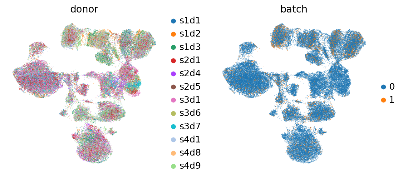
As we can see here, the cells of different donors are much more intermixed in the embedding than before (see plots from the Dimensionality Reduction chapter).
sc.pl.umap(mdata["prot"], color=["CD4-1", "CD8", "CD3"])
sc.pl.umap(mdata["prot"], color=["CD14-1", "CD16"])
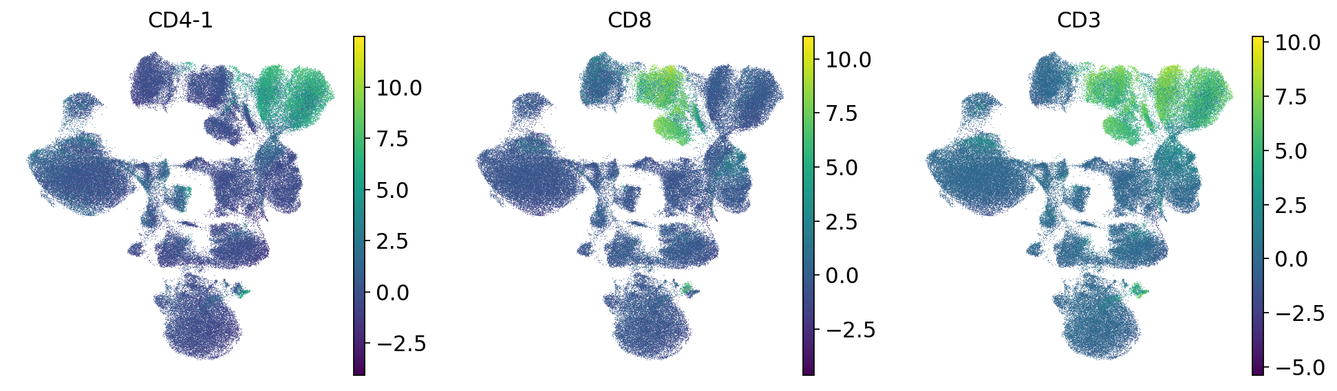
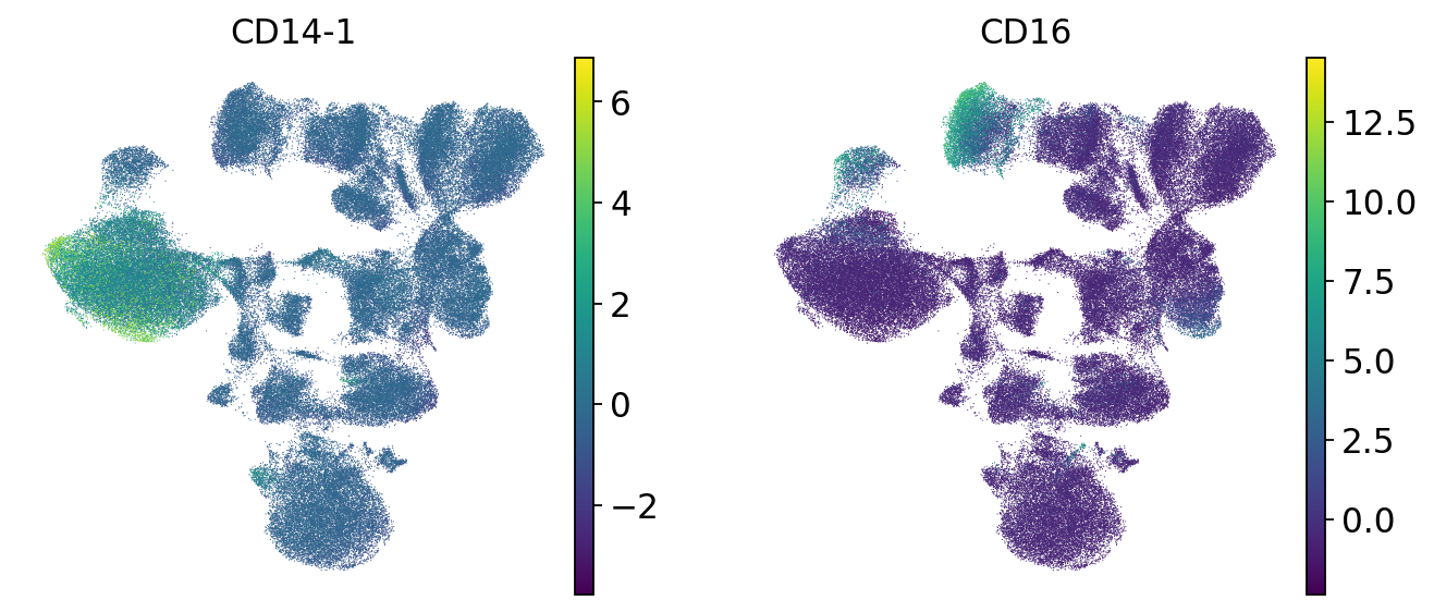
We check the expression of a few marker genes to confirm that separate cell types are still separate from each other. We can see that T cells still form a separate population that is further split into CD4 and CD8 T cells. Additionally, unlike before dimensionality reduction, now CD4 T cells form a discrete cluster where the donors are intermingled. Batch correction was therefore successful.
af_batch_correction = ln.Artifact.from_mudata(
    mdata,
    key="surface-protein/cite_batch_correction.h5mu",
    description="CITE-seq data after batch correction",
)
af_batch_correction.save()
ln.finish()
38.5. References#
Florian Ingelfinger, Nathan Levy, Can Ergen, Artemy Bakulin, Alexander Becker, Pierre Boyeau, Martin Kim, Diana Ditz, Jan Dirks, Jonas Maaskola, and others. Cytovi: deep generative modeling of antibody-based single cell technologies. bioRxiv, pages 2025–09, 2025.
Ilya Korsunsky, Nghia Millard, Jean Fan, Kamil Slowikowski, Fan Zhang, Kevin Wei, Yuriy Baglaenko, Michael Brenner, Po-ru Loh, and Soumya Raychaudhuri. Fast, sensitive and accurate integration of single-cell data with harmony. Nature Methods, 16(12):1289–1296, Dec 2019. URL: https://doi.org/10.1038/s41592-019-0619-0, doi:10.1038/s41592-019-0619-0.
Ye Zheng, Daniel P Caron, Ju Yeong Kim, Seong-Hwan Jun, Yuan Tian, Florian Mair, Kenneth D Stuart, Peter A Sims, and Raphael Gottardo. Adtnorm: robust integration of single-cell protein measurement across cite-seq datasets. Nature communications, 16(1):5852, 2025.
38.6. Contributors#
We gratefully acknowledge the contributions of:
38.6.2. Reviewers#
Lukas Heumos
Anna Schaar