3. Raw data processing#
Key takeaways
Accurate raw data processing transforms FASTQ files into a count matrix, enabling reliable single-cell sequencing analyses through read alignment, barcode correction, and UMI counting.
Environment setup
Install conda:
Before creating the environment, ensure that conda is installed on your system.
Save the yml content:
Copy the content from the yml tab into a file named
environment.yml.
Create the environment:
Open a terminal or command prompt.
Run the following command:
conda env create -f environment.yml
Activate the environment:
After the environment is created, activate it using:
conda activate <environment_name>
Replace
<environment_name>with the name specified in theenvironment.ymlfile. In the yml file it will look like this:name: <environment_name>
Verify the installation:
Check that the environment was created successfully by running:
conda env list
3.1. Motivation#
Raw data processing in single-cell sequencing converts sequencing machine output (so-called lane-demultiplexed FASTQ files) into readily analyzable representations such as a count matrix. This matrix represents the estimated number of distinct molecules derived from each gene per quantified cell, sometimes categorized by the inferred splicing status of each molecule (Fig. 3.1).
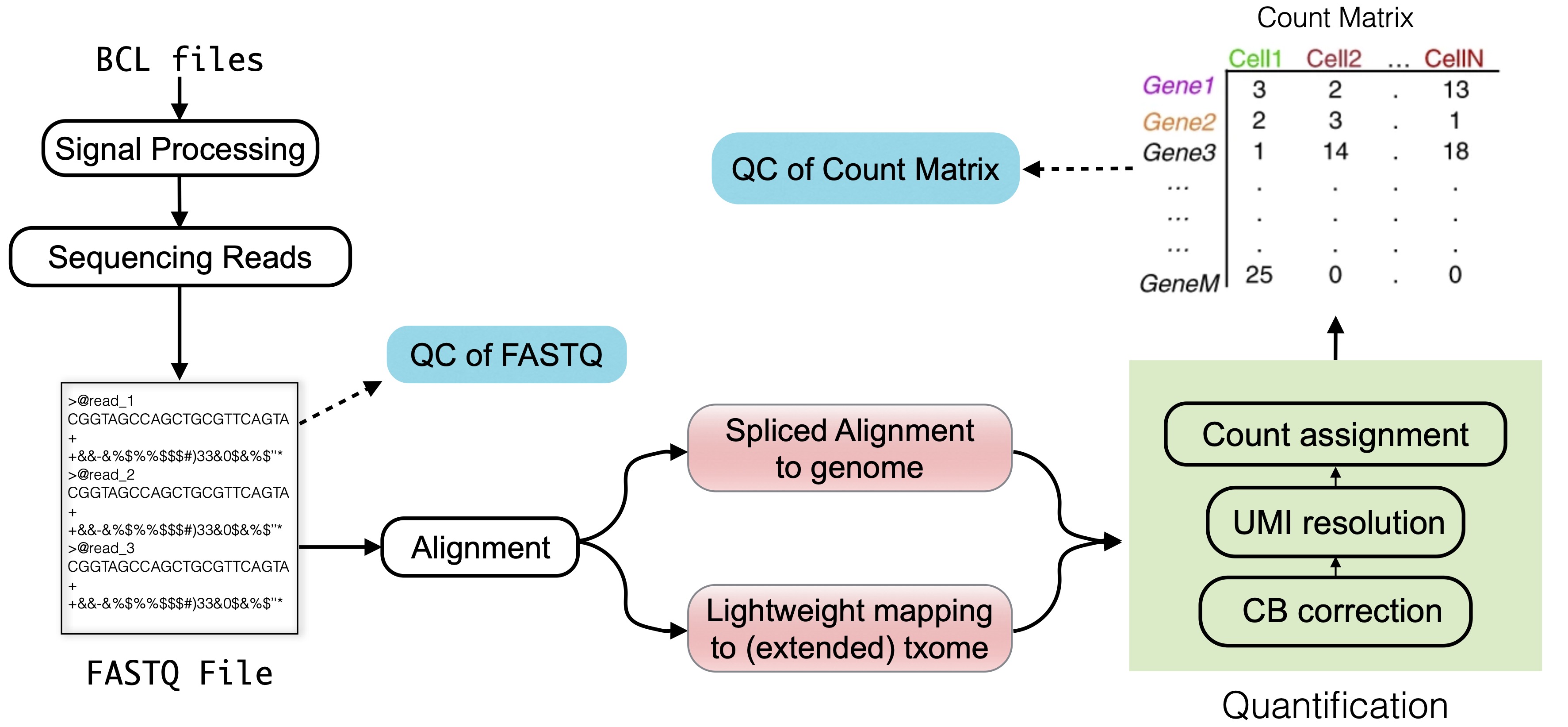
Fig. 3.1 An overview of the topics discussed in this chapter. In the plot, “txome” stands for transcriptome.#
The count matrix is the foundation for a wide range of scRNA-seq analyses [Zappia and Theis, 2021], including cell type identification or developmental trajectory inference. A robust and accurate count matrix is essential for reliable downstream analyses. Errors at this stage can lead to invalid conclusions and discoveries based on missed insights, or distorted signals in the data. Despite the straightforward nature of the input (FASTQ files) and the desired output (count matrix), raw data processing presents several technical challenges.
In this section, we focus on key steps of raw data processing:
Read alignment/mapping
Cell barcode (CB) identification and correction
Estimation of molecule counts through unique molecular identifiers (UMIs)
We also discuss the challenges and trade-offs involved in each step.
A note on preceding steps
The starting point for raw data processing is somewhat arbitrary. For this discussion, we treat lane-demultiplexed FASTQ files as the raw input. However, these files are derived from earlier steps, such as base calling and base quality estimation, which can influence downstream processing. For example, base-calling errors and index hopping [Farouni et al., 2020] can introduce inaccuracies in FASTQ data. These issues can be mitigated with computational approaches [Farouni et al., 2020] or experimental enhancements like dual indexing.
Here, we do not delve into the upstream processes, but consider the FASTQ files, derived from, e.g., BCL files via appropriate tools, as the raw input under consideration.
3.2. Raw data quality control#
After obtaining raw FASTQ files, it is important to evaluate the quality of the sequencing reads.
A quick and effective way to perform this is by using quality control (QC) tools like FastQC.
FastQC generates a detailed report for each FASTQ file, summarizing key metrics such as quality scores, base content, and other statistics that help identify potential issues arising from library preparation or sequencing.
While many modern single-cell data processing tools include some built-in quality checks—such as evaluating the N content of sequences or the fraction of mapped reads - it is still good practice to run an independent QC check.
For readers interested in what a typical FastQC report looks like, in the following toggle content, example reports for both high-quality and low-quality Illumina data provided by the FastQC manual webpage, along with the tutorials and descriptions from the RTSF at MSU, the HBC training program, and the QC Fail website are used to demonstrate the modules in the FastQC report.
Although these tutorials are not explicitly made for single-cell data, many of the results are still relevant for single-cell data, with a few caveats described below.
In the toggle section, all graphs, except specifically mentioned, are taken from the example reports on the FastQC manual webpage.
It is important to note that many QC metrics in FastQC reports are most meaningful only for biological reads—those derived from gene transcripts.
For single-cell datasets, such as 10x Chromium v2 and v3, this typically corresponds to read 2 (the files containing R2 in their filename), which contain transcript-derived sequences.
In contrast, technical reads, which contain barcode and UMI sequences, often do not exhibit biologically typical sequence or GC content.
However, certain metrics, like the fraction of N base calls, are still relevant for all reads.
Example FastQC Reports and Tutorials
0. Summary
The summary panel on the left side of the HTML report displays the module names along with symbols that provide a quick assessment of the module results.
However, FastQC applies uniform thresholds across all sequencing platforms and biological materials.
As a result, warnings (orange exclamation marks) or failures (red crosses) may appear for high-quality data, while questionable data might receive passes (green ticks).
Therefore, each module should be carefully reviewed before drawing conclusions about data quality.
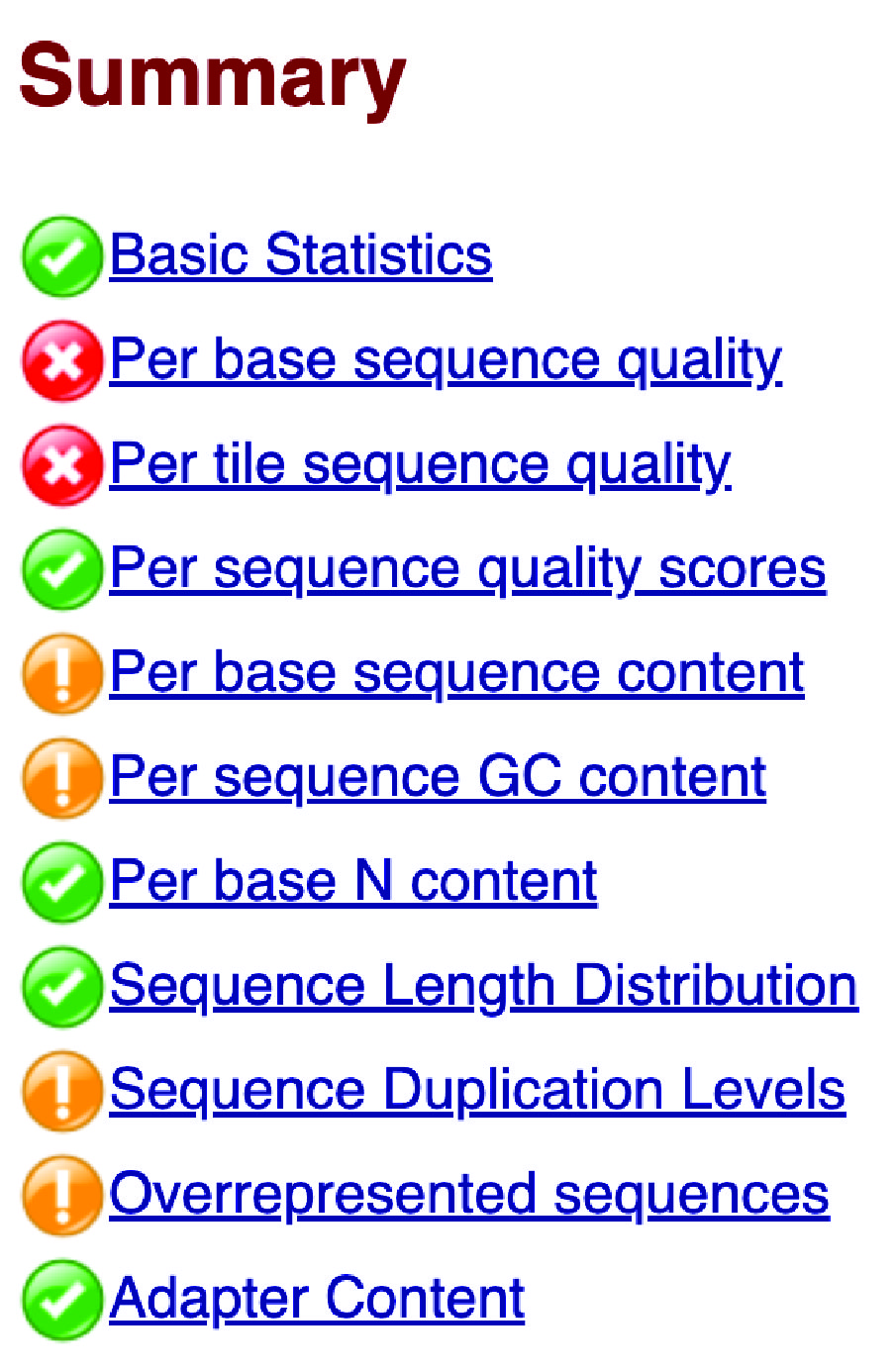
Fig. 3.2 The summary panel of a bad example.#
1. Basic statistics
The basic statistics module provides an overview of key information and statistics for the input FASTQ file, including the filename, total number of sequences, number of poor-quality sequences, sequence length, and the overall GC content (%GC) across all bases in all sequences. High-quality single-cell data typically have very few poor-quality sequences and exhibit a uniform sequence length. Additionally, the GC content should align with the expected GC content of the genome or transcriptome of the sequenced species.
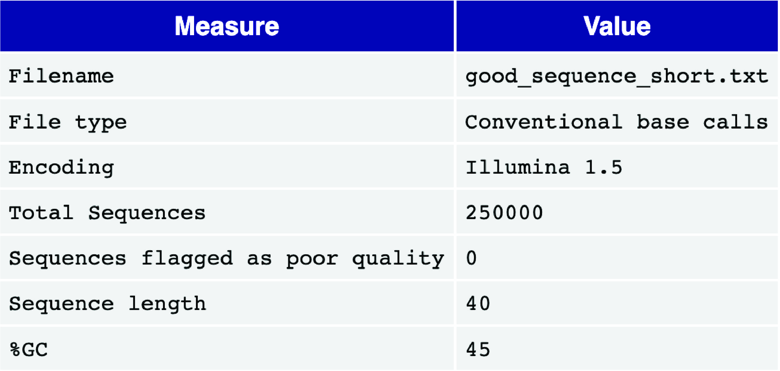
Fig. 3.3 A good basic statistics report example.#
2. Per base sequence quality
The per-base sequence quality view displays a box-and-whisker plot for each position in the read. The x-axis represents the positions within the read, while the y-axis shows the quality scores.
For high-quality single-cell data, the yellow boxes—representing the interquartile range of quality scores—should fall within the green area (indicating good quality calls). Similarly, the whiskers, which represent the 10th and 90th percentiles of the distribution, should also remain within the green area. It is common to observe a gradual drop in quality scores along the length of the read, with some base calls at the last positions falling into the orange area (reasonable quality) due to a decreasing signal-to-noise ratio, a characteristic of sequencing-by-synthesis methods. However, the boxes should not extend into the red area (poor quality calls).
If poor-quality calls are observed, quality trimming may be necessary. A more detailed explanation of sequencing error profiles can be found in the HBC training program.
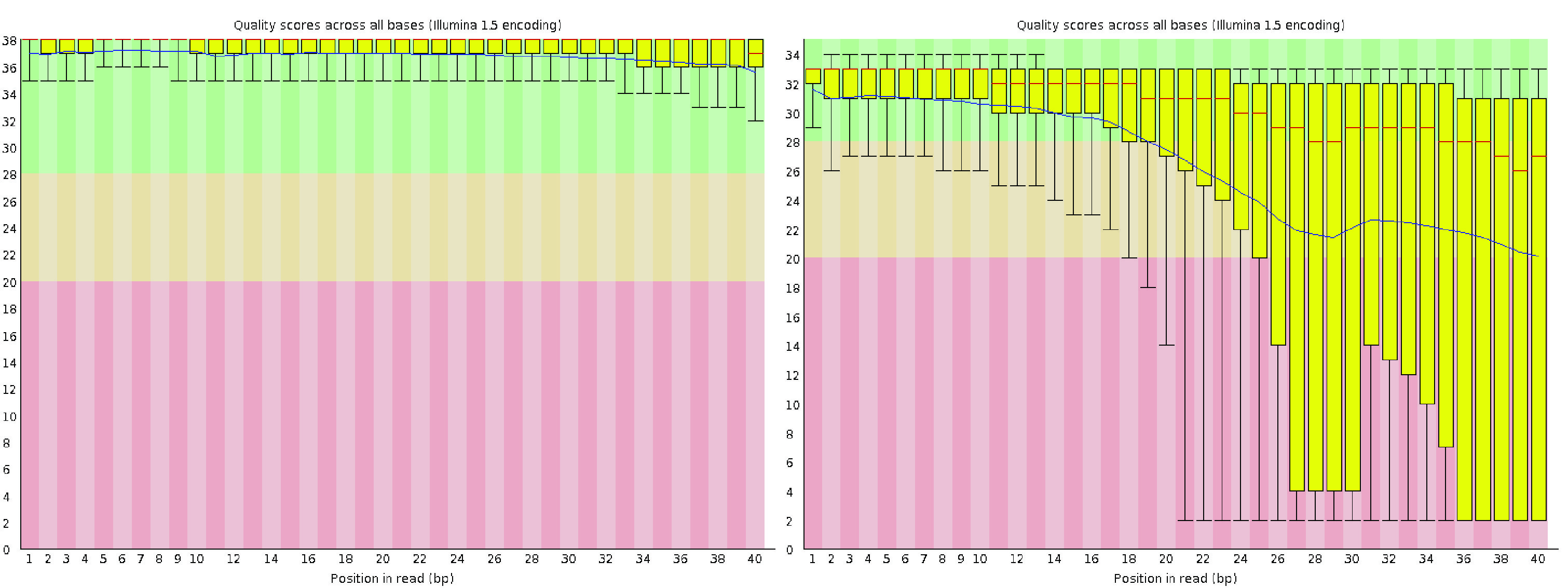
Fig. 3.4 A good (left) and a bad (right) per-read sequence quality graph.#
3. Per tile sequence quality
Using an Illumina library, the per-tile sequence quality plot highlights deviations from the average quality for reads across each tile(miniature imaging areas of the flowcell). The plot uses a color gradient to represent deviations, where warmer colors indicate larger deviations. High-quality data typically display a uniform blue color across the plot, indicating consistent quality across all tiles of the flowcell.
If warm colors appear in certain areas, it suggests that only part of the flowcell experienced poor quality.
This could result from transient issues during sequencing, such as bubbles passing through the flowcell or smudges and debris within the flowcell lane.
For further investigation, consult resources like QC Fail and the common reasons for warnings provided in the FastQC manual.
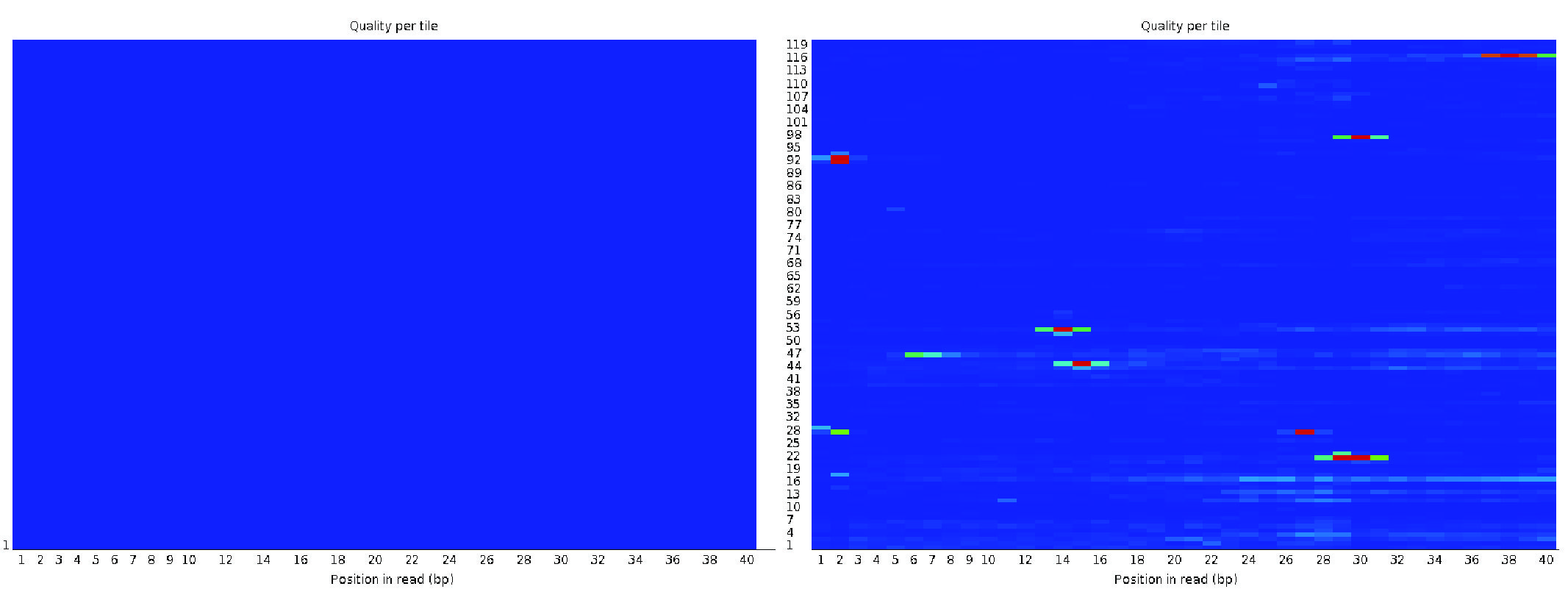
Fig. 3.5 A good (left) and a bad (right) per tile sequence quality view.#
4. Per sequence quality scores
The per-sequence quality score plot displays the distribution of average quality scores for each read in the file. The x-axis represents the average quality scores, while the y-axis shows the frequency of each score. For high-quality data, the plot should have a single peak near the high-quality end of the scale. If additional peaks appear, it may indicate a subset of reads with quality issues.
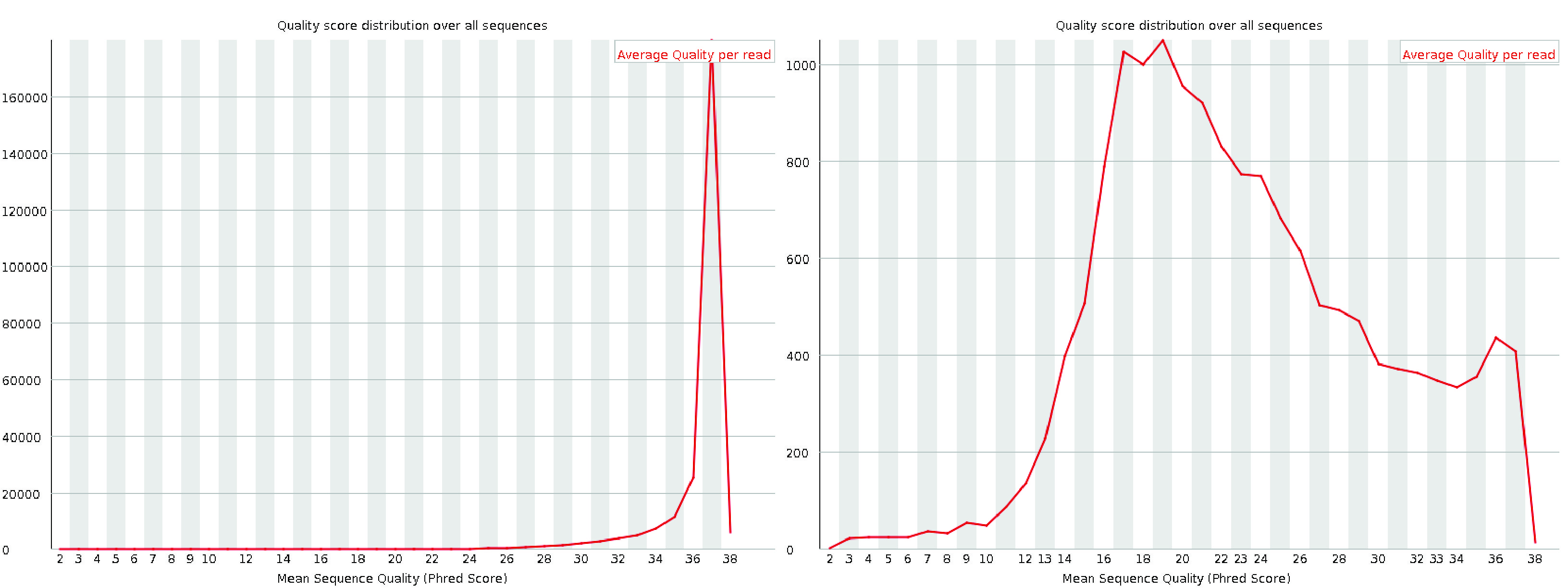
Fig. 3.6 A good (left) and a bad (right) per sequence quality score plot.#
5. Per base sequence content
The per-base sequence content plot shows the percentage of each nucleotide (A, T, G, and C) called at each base position across all reads in the file.
For single-cell data, it is common to observe fluctuations at the start of the reads.
This occurs because the initial bases represent the sequence of the priming sites, which are often not perfectly random.
This is a frequent occurrence in RNA-seq libraries, even though FastQC may flag it with a warning or failure, as noted on the QC Fail website.
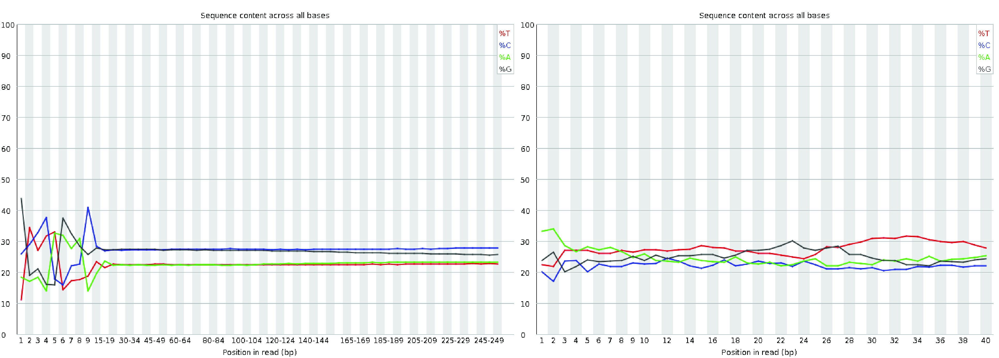
Fig. 3.7 A good (left) and bad (right) per base sequence content plot.#
6. Per sequence GC content
The per-sequence GC content plot displays the GC content distribution across all reads (in red) compared to a theoretical distribution (in blue).
The central peak of the observed distribution should align with the overall GC content of the transcriptome.
However, the observed distribution may appear wider or narrower than the theoretical one due to differences between the transcriptome’s GC content and the genome’s expected GC distribution.
Such variations are common and may trigger a warning or failure in FastQC, even if the data is acceptable.
A complex or irregular distribution in this plot, however, often indicates contamination in the library. It is also important to note that interpreting GC content in transcriptomics can be challenging. The expected GC distribution depends not only on the sequence composition of the transcriptome but also on gene expression levels in the sample, which are typically unknown beforehand. As a result, some deviation from the theoretical distribution is not unusual in RNA-seq data.
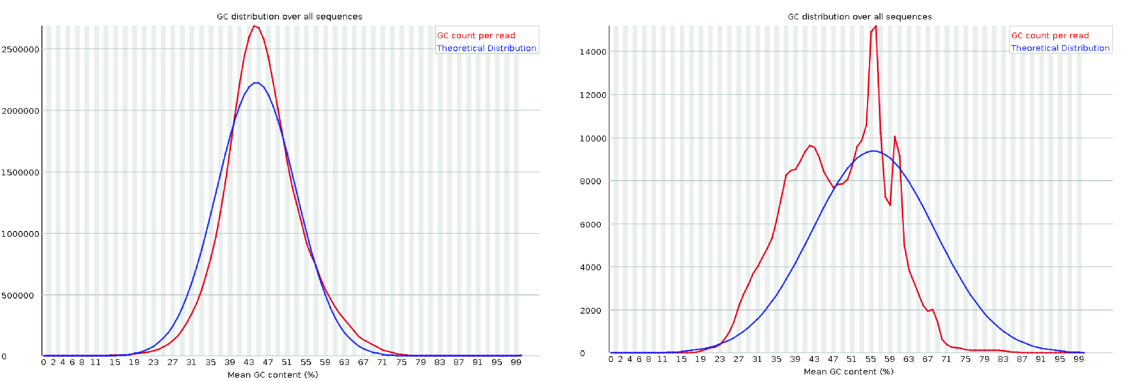
Fig. 3.8 A good (left) and a bad (right) per sequence GC content plot. The plot on the left is from the RTSF at MSU. The plot on the right is taken from the HBC training program.#
7. Per base N content
The per-base N content plot displays the percentage of bases at each position that were called as N, indicating that the sequencer lacked sufficient confidence to assign a specific nucleotide.
In a high-quality library, the N content should remain consistently at or near zero across the entire length of the reads.
Any noticeable non-zero N content may indicate issues with sequencing quality or library preparation.
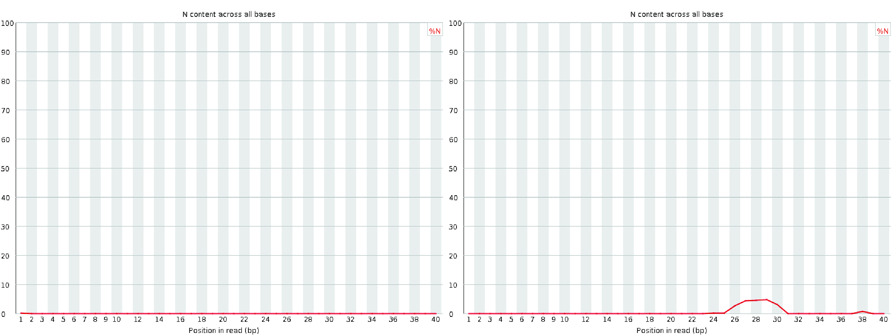
Fig. 3.9 A good (left) and a bad (right) per base N content plot.#
8. Sequence length distribution
The sequence length distribution graph displays the distribution of read lengths across all sequences in the file. For most single-cell sequencing chemistries, all reads are expected to have the same length, resulting in a single peak in the graph. However, if quality trimming was applied before the quality assessment, some variation in read lengths may be observed. Small differences in read lengths due to trimming are normal and should not be a cause for concern if expected.
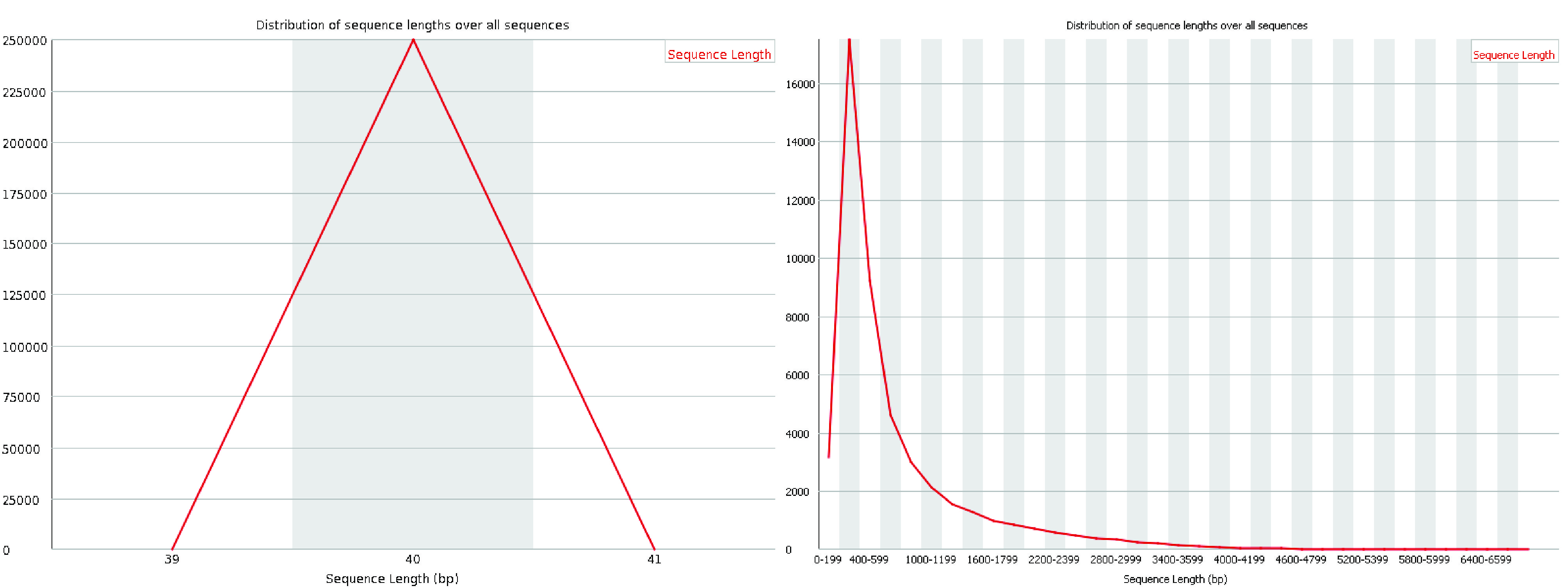
Fig. 3.10 A good (left) and a bad (right) sequence length distribution plot.#
9. Sequence duplication levels
The sequence duplication level plot illustrates the distribution of duplication levels for read sequences, represented by the blue line, both before and after deduplication.
In single-cell platforms, multiple rounds of PCR are typically required, and highly expressed genes naturally produce a large number of transcripts.
Additionally, since FastQC is not UMI-aware (i.e., it does not account for unique molecular identifiers), it is common for a small subset of sequences to show high duplication levels.
While this may trigger a warning or failure in this module, it does not necessarily indicate a quality issue with the data. However, the majority of sequences should still exhibit low duplication levels, reflecting a diverse and well-prepared library.
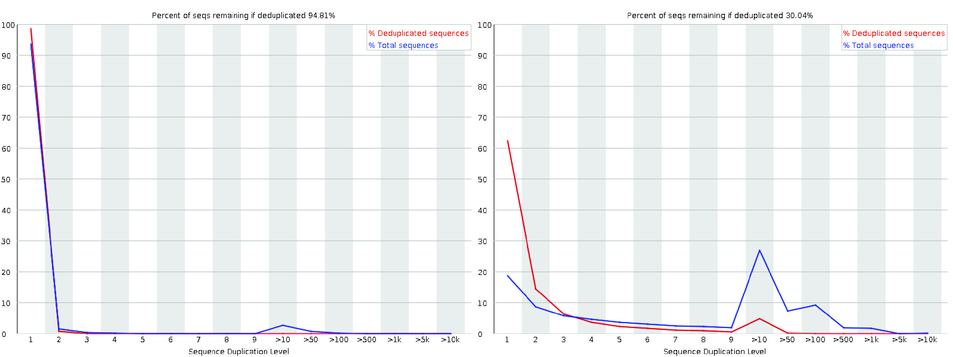
Fig. 3.11 A good (left) and a bad (right) per sequence duplication levels plot.#
10. Overrepresented sequences
The overrepresented sequences module identifies read sequences that constitute more than 0.1% of the total reads. In single-cell sequencing, some overrepresented sequences may arise from highly expressed genes amplified during PCR. However, the majority of sequences should not be overrepresented.
If the source of an overrepresented sequence is identified (i.e., not listed as “No Hit”), it could indicate potential contamination in the library from the corresponding source. Such cases warrant further investigation to ensure data quality.
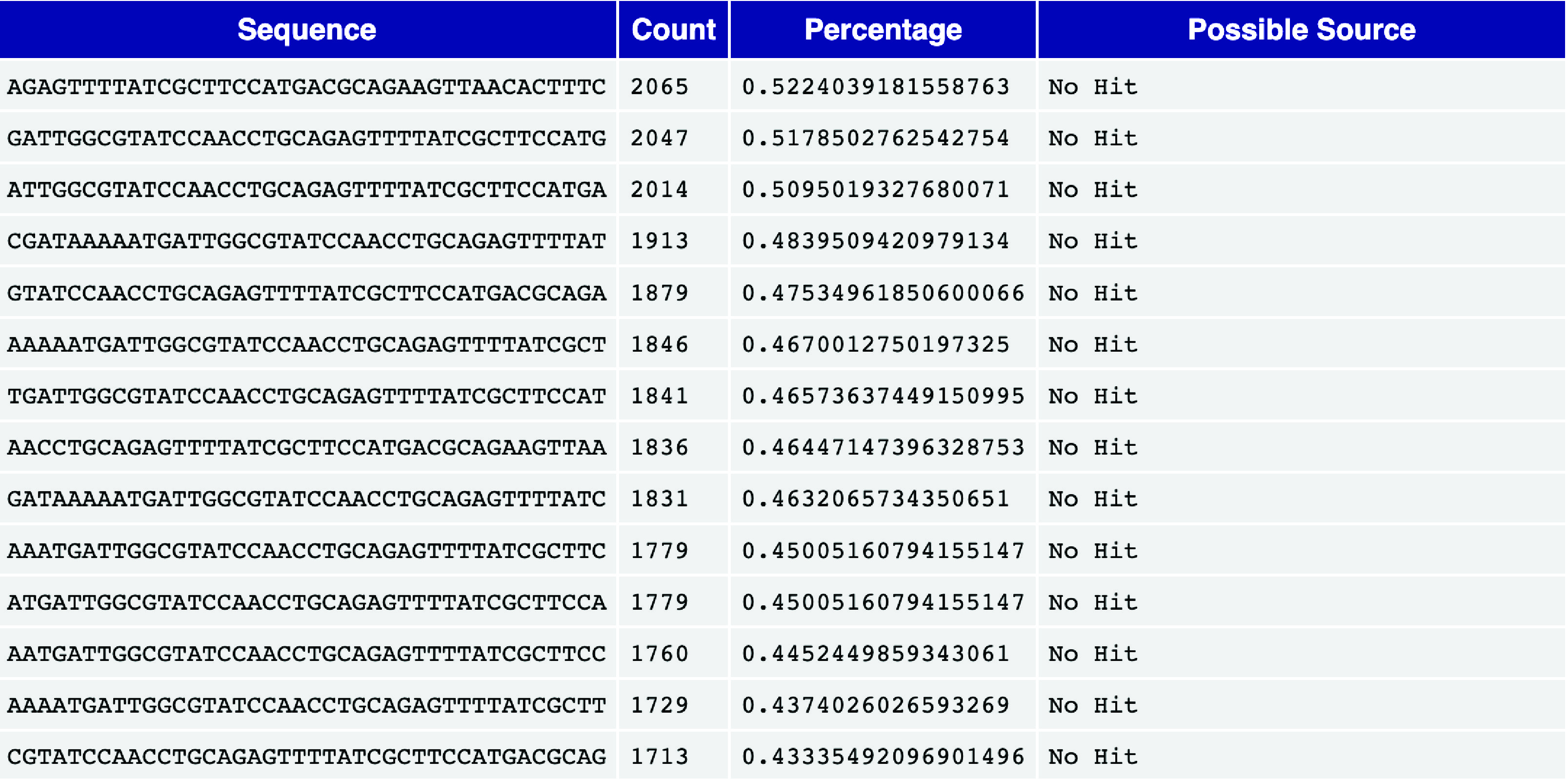
Fig. 3.12 An overrepresented sequence table.#
11. Adapter content
The adapter content module displays the cumulative percentage of reads containing adapter sequences at each base position. High levels of adapter sequences indicate incomplete removal of adapters during library preparation, which can interfere with downstream analyses. Ideally, no significant adapter content should be present in the data. If adapter sequences are abundant, additional trimming may be necessary to improve data quality.
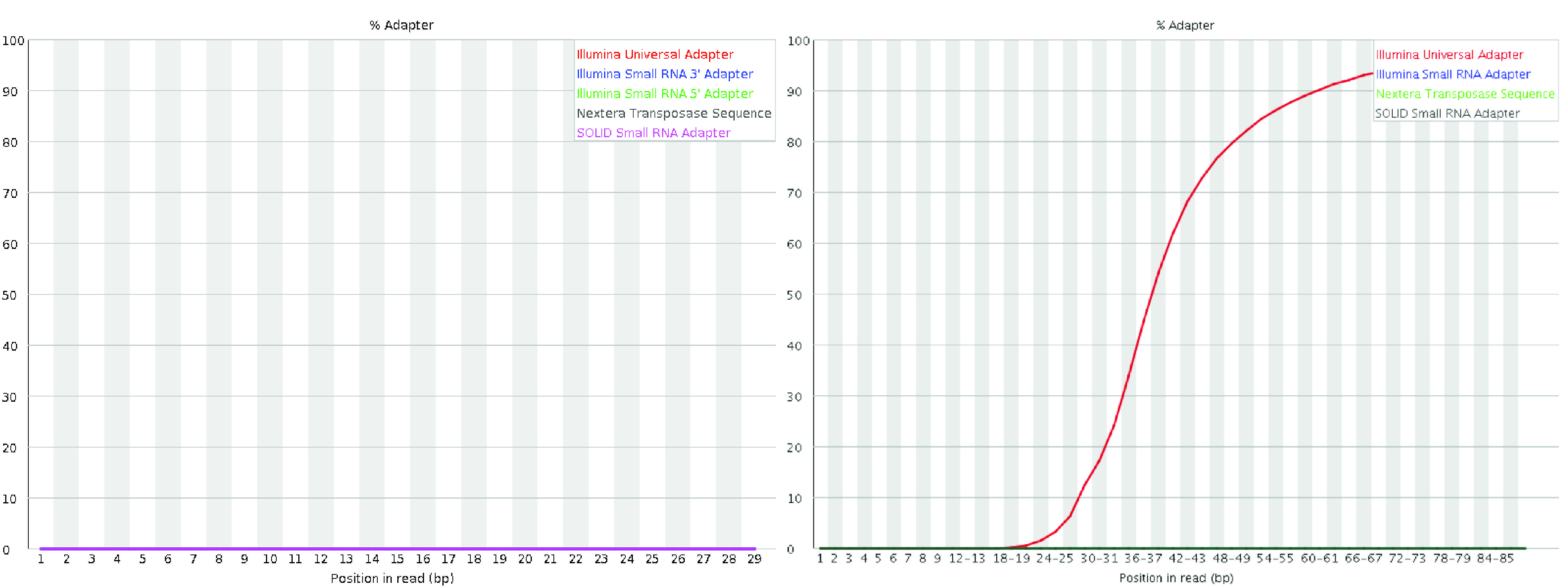
Fig. 3.13 A good (left) and a bad (right) per sequence quality score plot. The plot on the right is from the QC Fail website.#
Multiple FastQC reports can be combined into a single report using the tool MultiQC.
3.3. Alignment and mapping#
Mapping or Alignment is a critical step in single-cell raw data processing. It involves determining the potential loci of origin for each sequenced fragment, such as the genomic or transcriptomic locations that closely match the read sequence. This step is essential for correctly assigning reads to their source regions.
In single-cell sequencing protocols, the raw sequence files typically include:
Cell Barcodes (CB): Unique identifiers for individual cells.
Unique Molecular Identifiers (UMIs): Tags that distinguish individual molecules to account for amplification bias.
Raw cDNA Sequences: The actual read sequences generated from the molecules.
As the first step (Fig. 3.1), accurate mapping or alignment is crucial for reliable downstream analyses. Errors during this step, such as incorrect mapping of reads to transcripts or genes, can result in inaccurate or misleading count matrices.
While mapping read sequences to reference sequences far predates the development of scRNA-seq, the sheer scale of modern scRNA-seq datasets—often involving hundreds of millions to billions of reads—makes this step particularly computationally intensive. Many existing RNA-seq aligners are protocol-agnostic and do not inherently account for features specific to scRNA-seq, such as cell barcodes, UMIs, or their positions and lengths. As a result, additional tools are often required for steps like demultiplexing and UMI resolution [Smith et al., 2017].
To address the challenges of aligning and mapping scRNA-seq data, several specialized tools have been developed that handle the additional processing requirements automatically or internally. These tools include:
Cell Ranger(commercial software from 10x Genomics) [Zheng et al., 2017]zUMIs[Parekh et al., 2018]alevin[Srivastava et al., 2019]RainDrop[Niebler et al., 2020]kallisto|bustools[Melsted et al., 2021]STARsolo[Kaminow et al., 2021]alevin-fry[He et al., 2022]
These tools provide specialized capabilities for aligning scRNA-seq reads, parsing technical read content (e.g., cell barcodes and UMIs), demultiplexing, and UMI resolution. Although they offer simplified user interfaces, their internal methodologies differ significantly. Some tools generate traditional intermediate files, such as BAM files, which are processed further, while others operate entirely in memory or use compact intermediate representations to minimize input/output operations and reduce computational overhead.
While these tools vary in their specific algorithms, data structures, and trade-offs in time and space complexity, their approaches can generally be categorized along two axes:
The type of mapping they perform, and
The type of reference sequence against which they map reads.
3.3.1. Types of mapping#
We focus on three main types of mapping algorithms commonly used for mapping sc/snRNA-seq data: spliced alignment, contiguous alignment, and variations of lightweight mapping.
First, we distinguish between alignment-based approaches and lightweight mapping-based approaches (Fig. 3.14). Alignment-based methods use various heuristics to identify potential loci from which reads may originate and then score the best nucleotide-level alignment between the read and reference, typically using dynamic programming algorithms.
global alignment aligns the entirety of the query and reference sequences, while local alignment focuses on aligning subsequences. Short-read alignment often employs a semi-global approach, also known as “fitting” alignment, where most of the query aligns to a substring of the reference. Additionally, “soft-clipping” may be used to reduce penalties for mismatches, insertions, or deletions at the start or end of the read, achieved through “extension” alignment. While these variations modify the rules of the dynamic programming recurrence and traceback, they do not fundamentally alter its overall complexity.
Several sophisticated modifications and heuristics have been developed to enhance the practical efficiency of aligning genomic sequencing reads.
For example, banded alignment [Chao et al., 1992] is a popular heuristic used by many tools to avoid computing large portions of the dynamic programming table when alignment scores below a threshold are not of interest.
Other heuristics, like X-drop [Zhang et al., 2000] and Z-drop [Li, 2018], efficiently prune unpromising alignments early in the process.
Recent advances, such as wavefront alignment [Marco-Sola et al., 2020], marco2022optimal, enable the determination of optimal alignments in significantly reduced time and space, particularly when high-scoring alignments are present.
Additionally, much work has focused on optimizing data layout and computation to leverage instruction-level parallelism [Farrar, 2007, Rognes and Seeberg, 2000, Wozniak, 1997], and expressing dynamic programming recurrences in ways that facilitate data parallelism and vectorization, such as through difference encoding Suzuki and Kasahara [2018].
Most widely-used alignment tools incorporate these highly optimized, vectorized implementations.
In addition to the alignment score, the backtrace of the actual alignment that produces this score is often encoded as a CIGAR string (short for “Concise Idiosyncratic Gapped Alignment Report”).
This alphanumeric representation is typically stored in the SAM or BAM file output.
For example, the CIGAR string 3M2D4M indicates that the alignment has three matches or mismatches, followed by a deletion of length two (representing bases present in the reference but not the read), and then four more matches or mismatches.
Extended CIGAR strings can provide additional details, such as distinguishing between matches, mismatches, or insertions.
For instance, 3=2D2=2X encodes the same alignment as the previous example but specifies that the three bases before the deletion are matches, followed by two matched bases and two mismatched bases after the deletion.
A detailed description of the CIGAR string format can be found in the SAMtools manual or the SAM wiki page of UMICH.
Alignment-based approaches, though computationally expensive, provide a quality score for each potential mapping of a read.
This score allows them to distinguish between high-quality alignments and low-complexity or “spurious” matches between the read and reference.
These approaches include traditional “full-alignment” methods, such as those implemented in tools like STAR [Dobin et al., 2013] and STARsolo [Kaminow et al., 2021], as well as selective-alignment methods, like those in salmon [Srivastava et al., 2020] and alevin [Srivastava et al., 2019], which score mappings but skip the computation of the optimal alignment’s backtrace.
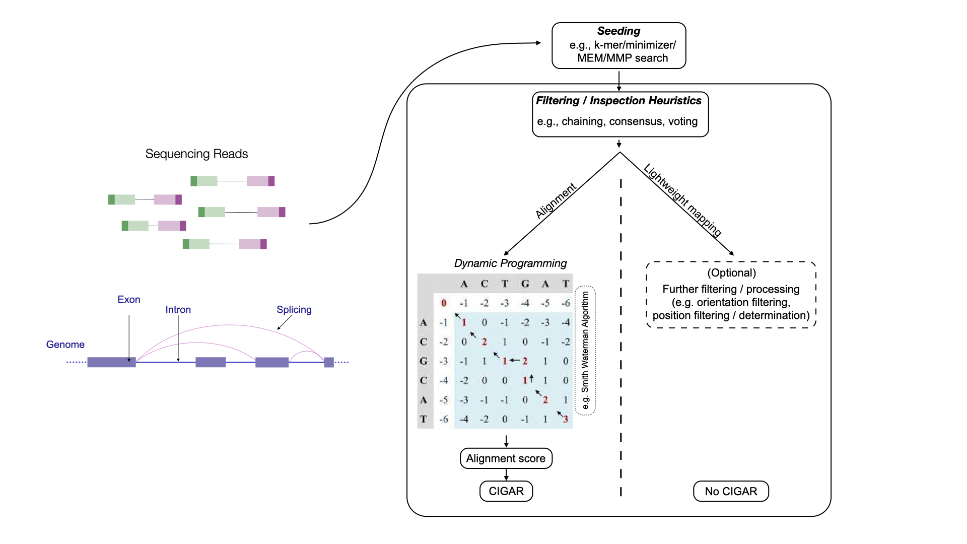
Fig. 3.14 An abstract overview of the alignment-based method and lightweight mapping-based method.#
Alignment-based approaches can be categorized into spliced-alignment and contiguous-alignment methods.
Spliced-alignment methods
Spliced-alignment methods allow a sequence read to align across multiple distinct segments of a reference, allowing potentially large gaps between aligned regions. These approaches are particularly useful for aligning RNA-seq reads to the genome, where reads may span splice junctions. In such cases, a contiguous sequence in the read may be separated by intron and exon subsequence in the reference, potentially spanning kilobases of sequence. Spliced alignment is especially challenging when only a small portion of a read overlaps a splice junction, as limited sequence information is available to accurately place the overhanging segment.
Contiguous-alignment methods
Contiguous-alignment methods require a continuous substring of the reference to align well with the read. While small insertions and deletions may be tolerated, large gaps—such as those in spliced alignments—are generally not allowed.
Alignment-based methods, such as spliced and contiguous alignment, can be distinguished from lightweight-mapping methods, which include approaches like pseudoalignment [Bray et al., 2016], quasi-mapping [Srivastava et al., 2016], and pseudoalignment with structural constraints [He et al., 2022].
Lightweight-mapping methods achieve significantly higher speed. However, they do not provide easily-interpretable score-based assessments to determine the quality of a match, making it more difficult to assess alignment confidence.
3.3.2. Mapping against different reference sequences#
In addition to selecting a mapping algorithm, choices can also be made regarding the reference sequence against which the reads are mapped. There are three main categories of reference sequences:
Full reference genome (typically annotated)
Annotated transcriptome
Augmented transcriptome
Currently, not all combinations of mapping algorithms and reference sequences are possible. For instance, lightweight-mapping algorithms do not yet support spliced mapping of reads against a reference genome.
3.3.2.1. Mapping to the full genome#
The first type of reference used for mapping is the entire genome of the target organism, typically with annotated transcripts considered during mapping.
Tools such as zUMIs [Parekh et al., 2018], Cell Ranger [Zheng et al., 2017], and STARsolo [Kaminow et al., 2021] follow this approach.
Since many reads originate from spliced transcripts, this method requires a splice-aware alignment algorithm capable of splitting alignments across one or more splice junctions.
A key advantage of this approach is that it accounts for reads arising from any location in the genome, not just those from annotated transcripts. Additionally, because a genome-wide index is constructed, there is minimal additional cost in reporting not only reads that map to known spliced transcripts but also those that overlap introns or align within non-coding regions, making this method equally effective for single-cell and single-nucleus data. Another benefit is that even reads mapping outside annotated transcripts, exons, or introns can still be accounted for, enabling post hoc augmentation of the quantified loci.
3.3.2.2. Mapping to the spliced transcriptome#
To reduce the computational overhead of spliced alignment to a genome, a widely adopted alternative is to use only the annotated transcript sequences as the reference. Since most single-cell experiments are conducted on model organisms like mouse or human, which have well-annotated transcriptomes, transcriptome-based quantification can achieve similar read coverage to genome-based methods.
Compared to the genome, transcriptome sequences are much smaller, significantly reducing the computational resources needed for mapping. Additionally, because splicing patterns are already represented in transcript sequences, this approach eliminates the need for complex spliced alignment. Instead, one can simply search for contiguous alignments or mappings for the read. Alternatively, reads can be mapped using contiguous alignments, making both alignment-based and lightweight-mapping techniques suitable for transcriptome references.
While these approaches significantly reduce the memory and time required for alignment and mapping, they fail to capture reads that arise from outside the spliced transcriptome. As a result, they are not suitable for processing single-nucleus data. Even in single-cell experiments, reads arising from outside of the spliced transcriptome can constitute a substantial fraction of all data, and there is growing evidence that such reads should be incorporated into subsequent analysis [Pool et al., 2022, 10x Genomics, 2021]. Additionally, when paired with lightweight-mapping methods, short sequences shared between the spliced transcriptome and the actual genomic regions that generated a read can lead to spurious mappings. This, in turn, may result in misleading and even biologically implausible gene expression estimates [Brüning et al., 2022, He et al., 2022, Kaminow et al., 2021].
3.3.2.3. Mapping to an augmented transcriptome#
To account for reads originating outside spliced transcripts, the spliced transcript sequences can be augmented with additional reference sequences, such as full-length unspliced transcripts or excised intronic sequences. This enables better, faster, and more memory-efficient mapping compared to full-genome alignment, while still capturing many reads that would otherwise be missed. More reads can be confidently assigned compared to using only the spliced transcriptome, and when combined with lightweight mapping approaches, spurious mappings can be significantly reduced [He et al., 2022]. Augmented transcriptomes are widely used in methods that do not map to the full genome, particularly for single-nucleus data processing and RNA velocity analysis [Soneson et al., 2021] (see RNA velocity). These augmented references can be constructed for all common methods that do not rely on spliced alignment to the full genome [He et al., 2022, Melsted et al., 2021, Srivastava et al., 2019].
3.4. Cell barcode correction#
Droplet-based single-cell segregation systems, such as those provided by 10x Genomics, have become an important tool for studying the cause and consequences of cellular heterogeneity. In this segregation system, the RNA material of each captured cell is extracted within a water-based droplet encapsulation along with a barcoded bead. These beads tag the RNA content of individual cells with unique oligonucleotides, called cell barcodes (CBs), that are later sequenced along with the fragments of the cDNAs that are reversely transcribed from the RNA content. The beads contain high-diversity DNA barcodes, allowing for parallel barcoding of a cell’s molecular content and in silico demultiplexing of sequencing reads into individual cellular bins.
A note on alignment orientation
Depending on the sample chemistry and user-defined processing options, not all sequenced fragments that align to the reference are necessarily considered for quantification and barcode correction. One commonly-applied criterion for filtering is alignment orientation. Specifically, certain chemistries specify protocols such that the aligned reads should only derive from (i.e. map back to) the underlying transcripts in a specific orientation. For example, in 10x Genomics 3’ Chromium chemistries, we expect the biological read to align to the underlying transcript’s forward strand, though anti-sense reads do exist [10x Genomics, 2021]. As a result, reads mapped in the reverse-complement orientation to the reference sequences may be ignored or filtered out based on user-defined settings. If a chemistry follows such a so-called “stranded” protocol, this should be documented.
3.4.1. Type of errors in barcoding#
The tag, sequence, and demultiplexing method used for single-cell profiling is generally effective. However, in droplet-based libraries, the number of observed cell barcodes (CBs) can differ significantly—often by several fold—from the number of originally encapsulated cells. This discrepancy arises from several key sources of error:
Doublets/multiplets: A single barcode may be associated with multiple cells, leading to an undercounting of cells.
Empty droplets: Some droplets contain no encapsulated cells, and ambient RNA can become tagged with a barcode and sequenced, resulting in overcounting of cells.
Sequence errors: Errors introduced during PCR amplification or sequencing can distort barcode counts, contributing to both under- and over-counting.
To address these issues, computational tools for demultiplexing RNA-seq reads into cell-specific bins use various diagnostic indicators to filter out artefactual or low-quality data. Numerous methods exist for removing ambient RNA contamination [Lun et al., 2019, Muskovic and Powell, 2021, Young and Behjati, 2020], detecting doublets [Bais and Kostka, 2019, DePasquale et al., 2019, McGinnis et al., 2019, Wolock et al., 2019], and correcting cell barcode errors based on nucleotide sequence similarity.
Several common strategies are used for cell barcode identification and correction.
Correction against a known list of potential barcodes: Certain chemistries, such as 10x Chromium, draw CBs from a known pool of potential barcode sequences. Thus, the set of barcodes observed in any sample is expected to be a subset of this known list, often called a “whitelist”. In this case, the standard approach assumes that:
Any barcode matching an entry in the known list is correct.
Any barcode not in the list is corrected by finding the closest match from the permit list, typically using Hamming distance or edit distance. This strategy allows for efficient barcode correction but has limitations. If a corrupted barcode closely resembles multiple barcodes in the permit list, its correction becomes ambiguous. For example, for a barcode taken from the 10x Chromium v3 permit list and mutated at a single position to a barcode not in the list, there is an \(\sim 81\%\) probability that it sits at hamming distance \(1\) from two or more barcodes in the permit list. The probability of such collisions can be reduced by considering correcting only against barcodes from the known permit list, which, themselves, occur exactly in the given sample (or even only those that occur exactly in the given sample above some nominal frequency threshold). Also, information such as the base quality at the “corrected” position can be used to potentially break ties in the case of ambiguous corrections. Yet, as the number of assayed cells increases, insufficient sequence diversity in the set of potential cell barcodes increases the frequency of ambiguous corrections, and reads tagged with barcodes having ambiguous corrections are most commonly discarded.
Knee or elbow-based methods: If a set of potential barcodes is unknown - or even if it is known, but one wishes to correct directly from the observed data itself without consulting an external list - one can use a method based on the observation that high-quality barcodes are those associated with the highest number of reads in the sample. To achieve this, one can construct a cumulative frequency plot where barcodes are sorted in descending order based on the number of distinct reads or UMIs they are associated with. Often, this ranked cumulative frequency plot will contain a “knee” or “elbow” – an inflection point that can be used to characterize frequently occurring barcodes from infrequent (and therefore likely erroneous) barcodes. Many methods exist for attempting to identify such an inflection point [He et al., 2022, Lun et al., 2019, Smith et al., 2017] as a likely point of discrimination between properly captured cells and empty droplets. Subsequently, the set of barcodes that appear “above” the knee can be treated as a permit list against which the rest of the barcodes may be corrected, as in the first method list above. Such an approach is flexible as it can be applied in chemistries that have an external permit list and those that don’t. Further parameters of the knee-finding algorithms can be altered to yield more or less restrictive selected barcode sets. Yet, such an approach can have certain drawbacks, like a tendency to be overly conservative and sometimes failing to work robustly in samples where no clear knee is present.
Filtering and correction based on an expected cell count: When barcode frequency distributions lack a clear knee or show bimodal patterns due to technical artifacts, barcode correction can be guided by a user-provided expected cell count. In such an approach, the user provides an estimate of the expected number of assayed cells. Then, the barcodes are ordered by descending frequency, the frequency \(f\) at a robust quantile index near the expected cell count is obtained, and all cells having a frequency within a small constant fraction of \(f\) (e.g., \(\ge \frac{f}{10}\)) are considered as valid barcodes. Again, the remaining barcodes are corrected against this valid list by attempting to correct uniquely to one of these valid barcodes based on sequence similarity.
Filtering based on a forced number of valid cells: The simplest approach, although potentially problematic, is for the user to manually specify the number of valid barcodes.
The user chooses an index in the sorted barcode frequency list.
All barcodes above this threshold are considered valid.
Remaining barcodes are corrected against this list using standard similarity-based correction methods. While this guarantees selection of at least n cells, it assumes that the chosen threshold accurately reflects the number of real cells. It is only reasonable if the user has a good reason to believe that the threshold frequency should be set around the provided index.
3.5. UMI resolution#
After cell barcode (CB) correction, reads have either been discarded or assigned to a corrected CB. Subsequently, we wish to quantify the abundance of each gene within each corrected CB.
Because of the amplification bias as discussed in Transcript quantification, reads must be deduplicated, based upon their UMI, to assess the true count of sampled molecules (Fig. 3.15). Additionally, several other complicating factors present challenges when attempting to perform this estimation.
The UMI deduplication step aims to identify the set of reads and UMIs derived from each original, pre-PCR molecule in each cell captured and sequenced in the experiment. The result of this process is to allocate a molecule count to each gene in each cell, which is subsequently used in the downstream analysis as the raw expression estimate for this gene. We refer to this process of looking at the collection of observed UMIs and their associated mapped reads and attempting to infer the original number of observed molecules arising from each gene as the process of UMI resolution.
To simplify the explanation, reads that map to a reference (e.g., a genomic locus of a gene) are referred to as the reads of that reference, and their UMI tags are called the UMIs of that reference. The set of reads associated with a specific UMI is referred to as the reads of that UMI.
A read can be tagged by only one UMI but may belong to multiple references if it maps to more than one. Additionally, since molecule barcoding in scRNA-seq is typically isolated and independent for each cell (aside from the previously discussed challenges in resolving cell barcodes), UMI resolution will be explained for a single cell without loss of generality. This same procedure is generally applied to all cells independently.
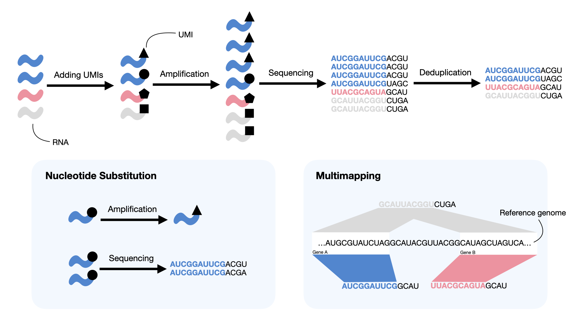
Fig. 3.15 UMIs reduce PCR amplification bias by tracking original molecules, but can be affected by different types of errors (blue boxes). Nucleotide substitutions in UMI tags may occur during amplification or sequencing. Multimapping can arise when reads sharing the same UMI are mapped to different genes (blue and red), when a single read maps to multiple genes (gray), or both.#
3.5.1. The need for UMI resolution#
In the ideal case, where the correct (unaltered) UMIs tag reads, the reads of each UMI uniquely map to a common reference gene, and there is a bijection between UMIs and pre-PCR molecules. Consequently, the UMI deduplication procedure is conceptually straightforward: the reads of a UMI are the PCR duplicates from a single pre-PCR molecule. The number of captured and sequenced molecules of each gene is the number of distinct UMIs observed for this gene.
However, the problems encountered in practice make the simple rules described above insufficient for identifying the gene origin of UMIs in general and necessitate the development of more sophisticated models (Fig. 3.15):
Errors in UMIs: These occur when the sequenced UMI tag of reads contains errors introduced during PCR or the sequencing process. Common UMI errors include nucleotide substitutions during PCR and read errors during sequencing. Failing to address such UMI errors can inflate the estimated number of molecules [Smith et al., 2017, Ziegenhain et al., 2022].
Multimapping: This issue arises in cases where a read or UMI belongs to multiple references (e.g., multi-gene reads/UMIs). This happens when different reads of a UMI map to different genes, when a read maps to multiple genes, or both. The consequence of this issue is that the gene origin of the multi-gene reads/UMIs is ambiguous, which results in uncertainty about the sampled pre-PCR molecule count of those genes. Simply discarding multi-gene reads/UMIs can lead to a loss of data or a biased estimate among genes that tend to produce multimapping reads, such as sequence-similar gene families [Srivastava et al., 2019].
A Note on UMI Errors
UMI errors, especially those due to nucleotide substitutions and miscallings, are prevalent in single-cell experiments. Smith et al. [2017] establish that the average number of bases different (edit distance) between the observed UMI sequences in the tested single-cell experiments is lower than randomly sampled UMI sequences, and the enrichment of low edit distances is well correlated with the degree of PCR amplification. Multimapping also exists in single-cell data and, depending upon the gene being considered, can occur at a non-trivial rate. Srivastava et al. [2019] show that discarding the multimapping reads can negatively bias the predicted molecule counts.
There exist other challenges that we do not focus upon here, such as “convergent” and “divergent” UMI collisions. We consider the case where the same UMI is used to tag two different pre-PCR molecules arising from the same gene, in the same cell, as a convergent collision. When two or more distinct UMIs arise from the same pre-PCR molecule, e.g., due to the sampling of multiple priming sites from this molecule, we consider this a divergent collision. We expect convergent UMI collisions to be rare and, therefore, their effect typically small. Further, transcript-level mapping information can sometimes be used to resolve such collisions [Srivastava et al., 2019]. Divergent UMI collisions occur primarily among introns of unspliced transcripts [10x Genomics, 2021], and approaches to addressing the issues they raise are an area of active research [Gorin and Pachter, 2021, 10x Genomics, 2021].
Given that the use of UMIs is near ubiquitous in high-throughput scRNA-seq protocols and the fact that addressing these errors improves the estimation of gene abundances, there has been much attention paid to the problem of UMI resolution in recent literature [Bose et al., 2015, He et al., 2022, Islam et al., 2013, Kaminow et al., 2021, Macosko et al., 2015, Melsted et al., 2021, Orabi et al., 2018, Parekh et al., 2018, Smith et al., 2017, Srivastava et al., 2019, Tsagiopoulou et al., 2021].
Graph-based UMI resolution
Graph-based UMI resolution
As a result of the problems that arise when attempting to resolve UMIs, many methods have been developed to address the problem of UMI resolution. While there are a host of different approaches for UMI resolution, we will focus on a framework for representing problem instances, modified from a framework initially proposed by Smith et al. [2017], that relies upon the notion of a UMI graph. Each connected component of this graph represents a sub-problem wherein certain subsets of UMIs are collapsed (i.e., resolved as evidence of the same pre-PCR molecule). Many popular UMI resolution approaches can be interpreted in this framework by simply modifying precisely how the graph is refined and how the collapse or resolution procedure carried out over this graph works.
In the context of single-cell data, a UMI graph \(G(V,E)\) is a directed graph with a node set \(V\) and an edge set \(E\). Each node \(v_i \in V\) represents an equivalence class (EC) of reads, and the edge set \(E\) encodes the relationship between the ECs. The equivalence relation \(\sim_r\) defined on reads is based on their UMI and mapping information. We say reads \(r_x\) and \(r_y\) are equivalent, \(r_x \sim_r r_y\), if and only if they have identical UMI tags and map to the same set of references. UMI resolution approaches may define a “reference” as a genomic locus [Smith et al., 2017], transcript [He et al., 2022, Srivastava et al., 2019] or gene [Kaminow et al., 2021, Zheng et al., 2017].
In the UMI graph framework, a UMI resolution approach can be divided into three major steps: defining nodes, defining adjacency relationships, and resolving components. Each of these steps has different options that can be modularly composed by different approaches. Additionally, these steps may sometimes be preceded (and/or followed) by filtering steps designed to discard or heuristically assign (by modifying the set of reference mappings reported) reads and UMIs exhibiting certain types of mapping ambiguity.
Defining nodes
As described above, a node \(v_i \in V\) is an equivalence class of reads. Therefore, \(V\) can be defined based on the full or filtered set of mapped reads and their associated uncorrected UMIs. All reads that satisfy the equivalence relation \(\sim_r\) based on their reference set and UMI tag are associated with the same vertex \(v \in V\). An EC is a multi-gene EC if its UMI is a multi-gene UMI. Some approaches will avoid the creation of such ECs by filtering or heuristically assigning reads prior to node creation, while other approaches will retain and process these ambiguous vertices and attempt and resolve their gene origin via parsimony, probabilistic assignment, or based on a related rule or model [He et al., 2022, Kaminow et al., 2021, Srivastava et al., 2019].
Defining the adjacency relationship
After creating the node set \(V\) of a UMI graph, the adjacency of nodes in \(V\) is defined based on the distance, typically the Hamming or edit distance, between their UMI sequences and, optionally, the content of their associated reference sets.
Here we define the following functions on the node \(v_i \in V\):
\(u(v_i)\) is the UMI tag of \(v_i\).
\(c(v_i) = |v_i|\) is the cardinality of \(v_i\), i.e., the number of reads associated with \(v_i\) that are equivalent under \(\sim_r\).
\(m(v_i)\) is the reference set encoded in the mapping information, for \(v_i\).
\(D(v_i, v_j)\) is the distance between \(u(v_i)\) and \(u(v_j)\), where \(v_j \in V\).
Given these function definitions, any two nodes \(v_i, v_j \in V\) will be incident with a bi-directed edge if and only if \(m(v_i) \cap m(v_j) \ne \emptyset\) and \(D(v_i,v_j) \le \theta\), where \(\theta\) is a distance threshold and is often set as \(\theta=1\) [Kaminow et al., 2021, Smith et al., 2017, Srivastava et al., 2019]. Additionally, the bi-directed edge might be replaced by a directed edge incident from \(v_i\) to \(v_j\) if \(c(v_i) \ge 2c(v_j) -1\) or vice versa [Smith et al., 2017, Srivastava et al., 2019]. Though these edge definitions are among the most common, others are possible, so long as they are completely defined by the \(u\), \(c\), \(m\), and \(D\) functions. With \(V\) and \(E\) in hand, the UMI graph \(G = (V,E)\) is now defined.
Defining the graph resolution approach
Given the defined UMI graph, many different resolution approaches may be applied. A resolution method may be as simple as finding the set of connected components, clustering the graph, greedily collapsing nodes or contracting edges [Smith et al., 2017], or searching for a cover of the graph by structures following certain rules (e.g., monochromatic arboresences [Srivastava et al., 2019]) to reduce the graph. As a result, each node in the reduced UMI graph, or each element in the cover in the case that the graph is not modified dynamically, represents a pre-PCR molecule. The collapsed nodes or covering sets are regarded as the PCR duplicates of that molecule.
Different rules for defining the adjacency relationship and different approaches for graph resolution itself can seek to preserve different properties and can define a wide variety of distinct overall UMI resolution approaches. For approaches that probabilistically resolve ambiguity caused by multimapping, the resolved UMI graph may contain multi-gene equivalence classes (ECs), with their gene origins determined in the next step.
Other UMI resolution approaches exist, for example, the reference-free model [Tsagiopoulou et al., 2021] and the method of moments [Melsted et al., 2021], but they may not be easily represented in this framework and are not discussed in further detail here.
3.5.1.1. Quantification#
The last step in UMI resolution is quantifying the abundance of each gene using the resolved UMI graph. For approaches that discard multi-gene ECs, the molecule count vector for the genes in the current cell being processed (or count vector for short) is generated by counting the number of ECs labeled with each gene. On the other hand, approaches that process, rather than discard, multi-gene ECs usually resolve the ambiguity by applying some statistical inference procedure. For example, Srivastava et al. [2019] introduce an expectation-maximization (EM) approach for probabilistically assigning multi-gene UMIs, and related EM algorithms have also been introduced as optional steps in subsequent tools [He et al., 2022, Kaminow et al., 2021, Melsted et al., 2021]. In this model, the collapsed-EC-to-gene assignments are latent variables, and the deduplicated molecule count of genes are the main parameters. Intuitively, evidence from gene-unique ECs will be used to help probabilistically apportion the multi-gene ECs. The EM algorithm seeks the parameters that together have the (locally) highest likelihood of generating the observed ECs.
Usually, the UMI resolution and quantification process described above will be performed separately for each cell, represented by a corrected CB, to create a complete count matrix for all genes in all cells. However, the relative paucity of per-cell information in high-throughput single-cell samples limits the evidence available when performing UMI resolution, which in turn limits the potential efficacy of model-based solutions like the statistical inference procedure described above.
3.6. Count matrix quality control#
Once a count matrix has been generated, it is important to perform a quality control (QC) assessment. There are several distinct assessments that generally fall under the rubric of quality control. Basic global metrics are often recorded and reported to help assess the overall quality of the sequencing measurement itself. These metrics consist of quantities such as the total fraction of mapped reads, the distribution of distinct UMIs observed per cell, the distribution of UMI deduplication rates, the distribution of detected genes per cell, etc. These and similar metrics are often recorded by the quantification tools themselves [He et al., 2022, Kaminow et al., 2021, Melsted et al., 2021, Zheng et al., 2017] since they arise naturally and can be computed during the process of read mapping, cell barcode correction, and UMI resolution. Likewise, there exist several tools to help organize and visualize these basic metrics, such as the Loupe browser, alevinQC, or a kb_python report, depending upon the quantification pipeline being used. Beyond these basic global metrics, at this stage of analysis, QC metrics are designed primarily to help determine which cells (CBs) have been sequenced “successfully”, and which exhibit artifacts that warrant filtering or correction.
In the following toggle section, we discuss an example alevinQC report taken from the alevinQC manual webpage.
Once alevin or alevin-fry quantifies the single-cell data, the quality of the data can be assessed through the R package alevinQC.
The alevinQC report can be generated in PDF format or as R/Shiny applications, which summarizes various components of the single-cell library, such as reads, CBs, and UMIs.
1. Metadata and summary tables
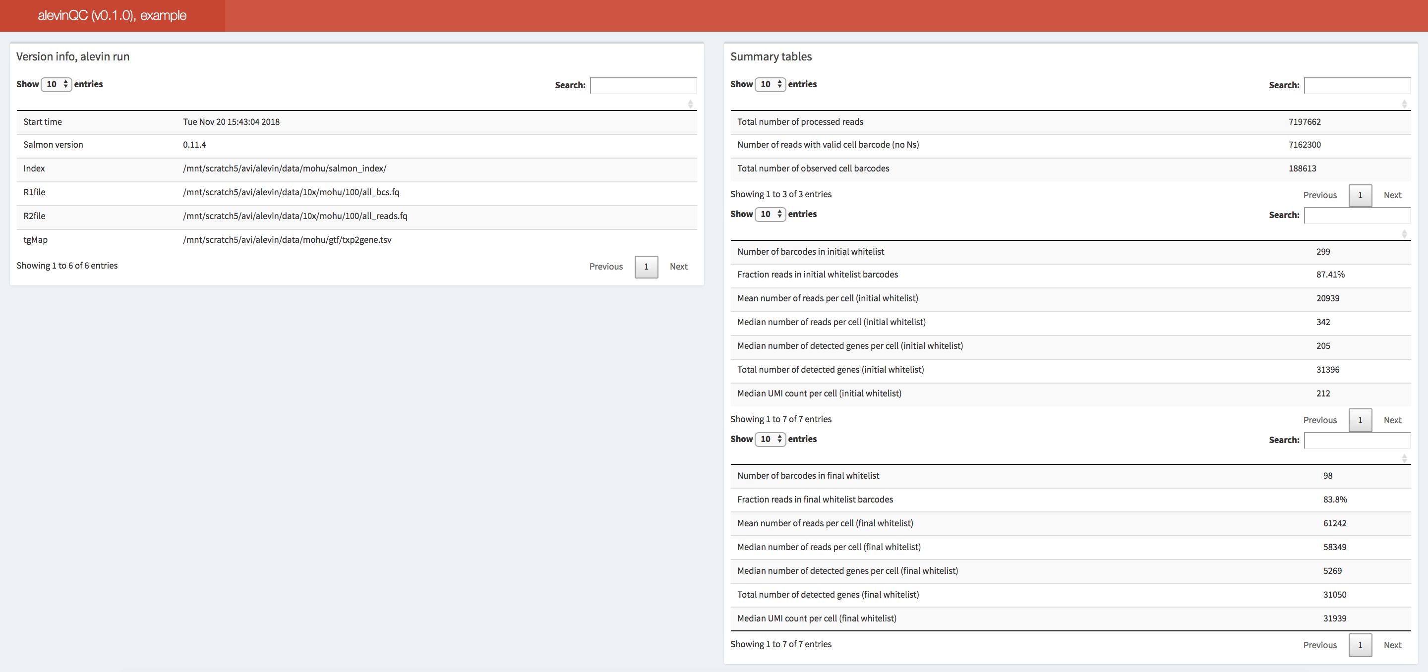
Fig. 3.16 An example of the summary section of an alevinQC report.#
The first section of an alevinQC report shows a summary of the input files and the processing result, among which, the top left table displays the metadata provided by alevin (or alevin-fry) for the quantification results.
For example, this includes the time of the run, the version of the tool, and the path to the input FASTQ and index files.
The top right summary table provides the summary statistics for various components of the single-cell library, for example, the number of sequencing reads, the number of selected cell barcodes at various levels of filtering, and the total number of deduplicated UMIs.
2. Knee plot, initial whitelist determination
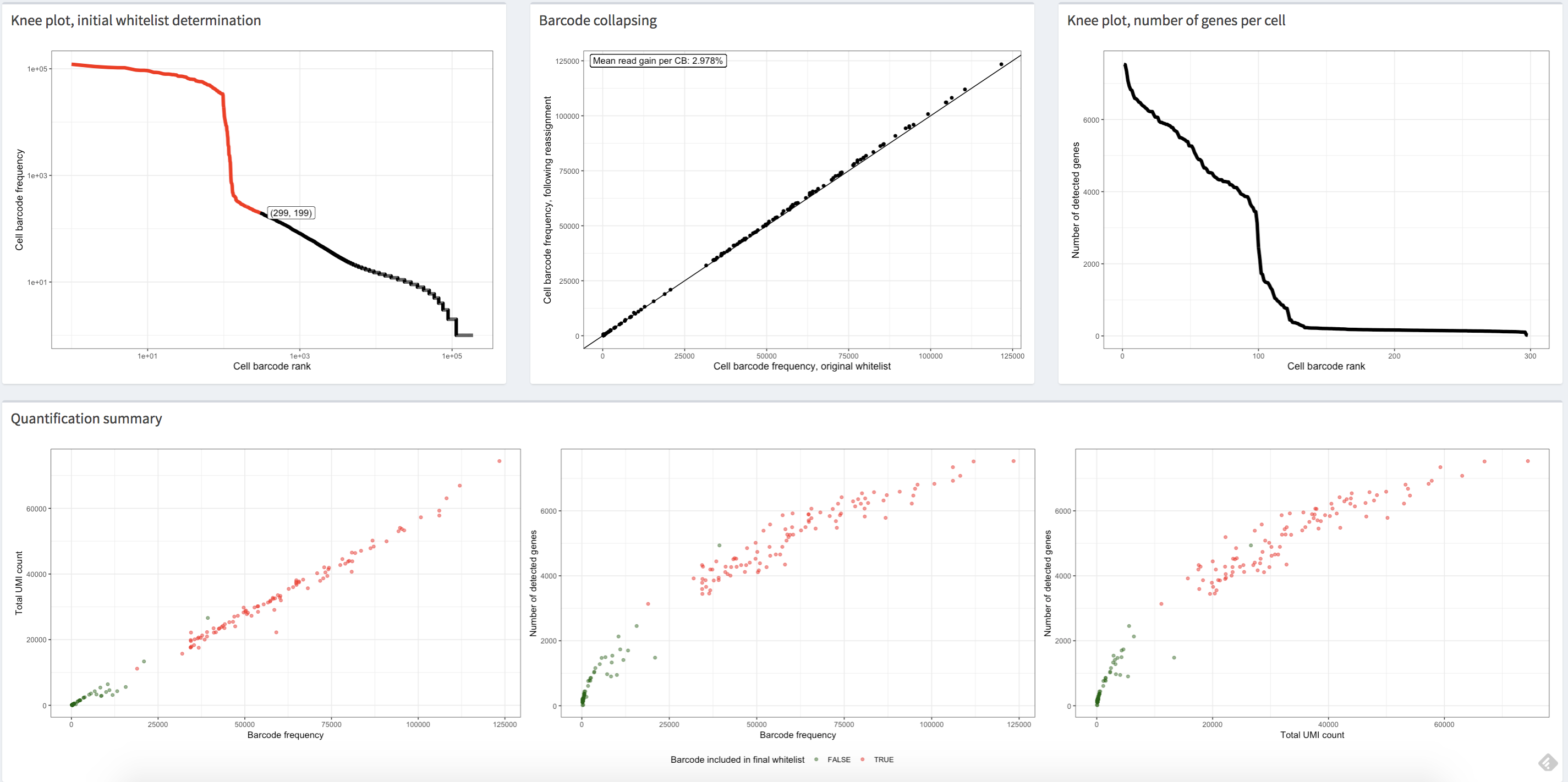
Fig. 3.17 The figure shows the plots in the alevinQC report of an example single-cell dataset, of which the cells are filtered using the “knee” finding method. Each dot represents a corrected cell barcode with its corrected profile.#
The first (top left) view in Fig. 3.17 shows the distribution of cell barcode frequency in decreasing order. In all plots shown above, each point represents a corrected cell barcode, with its x-coordinate corresponding to its cell barcode frequency rank. In the top left plot, the y-coordinate corresponds to the observed frequency of the corrected barcode. Generally, this plot shows a “knee”-like pattern, which can be used to identify the initial list of high-quality barcodes. The red dots in the plot represent the cell barcodes selected as the high-quality cell barcodes in the case that “knee”-based filtering was applied. In other words, these cell barcodes contain a sufficient number of reads to be deemed high-quality and likely derived from truly present cells. Suppose an external permit list is passed in the CB correction step, which implies no internal algorithm was used to distinguish high-quality cell barcodes. In that case, all dots in the plot will be colored red, as all these corrected cell barcodes are processed throughout the raw data processing pipeline and reported in the gene count matrix. One should be skeptical of the data quality if the frequency is consistently low across all cell barcodes.
3. Barcode collapsing
After identification of the barcodes that will be processed, either through an internal threshold (e.g., from the “knee”-based method) or through external whitelisting, alevin (or alevin-fry) performs cell barcode sequence correction.
The barcode collapsing plot, the upper middle plot in the Fig. 3.17, shows the number of reads assigned to a cell barcode after sequence correction of the cell barcodes versus prior to correction.
Generally, we would see that all points fall close to the line representing \(x = y\), which means that the reassignments in CB correction usually do not drastically change the profile of the cell barcodes.
4. Knee Plot, number of genes per cell
The upper right plot in Fig. 3.17 shows the distribution of the number of observed genes of all processed cell barcodes. Generally, a mean of \(2,000\) genes per cell is considered modest but reasonable for the downstream analyses. One should double-check the quality of the data if all cells have a low number of observed genes.
5. Quantification summary
Finally, a series of quantification summary plots, the bottom plots in Fig. 3.17, compare the cell barcode frequency, the total number of UMIs after deduplication and the total number of non-zero genes using scatter plots. In general, in each plot, the plotted data should demonstrate a positive correlation, and, if high-quality filtering (e.g., knee filtering) has been performed, the high-quality cell barcodes should be well separated from the rest. Moreover, one should expect all three plots to convey similar trends. If using an external permit list, all the dots in the plots will be colored red, as all these cell barcodes are processed and reported in the gene count matrix. Still, we should see the correlation between the plots and the separation of the dots representing high-quality cells to others. If all of these metrics are consistently low across cells or if these plots convey substantially different trends, then one should be concerned about the data quality.
3.6.1. Empty droplet detection#
One of the first QC steps is determining which cell barcodes correspond to “high-confidence” sequenced cells. It is common in droplet-based protocols [Macosko et al., 2015] that certain barcodes are associated with ambient RNA instead of the RNA of a captured cell. This happens when droplets fail to capture a cell. These empty droplets still tend to produce sequenced reads, although the characteristics of these reads look markedly different from those associated with barcodes corresponding to properly captured cells. Many approaches exist to assess whether a barcode likely corresponds to an empty droplet or not. One simple method is to examine the cumulative frequency plot of the barcodes, in which barcodes are sorted in descending order of the number of distinct UMIs with which they are associated. This plot often contains a “knee” that can be identified as a likely point of discrimination between properly captured cells and empty droplets [He et al., 2022, Smith et al., 2017]. While this “knee” method is intuitive and can often estimate a reasonable threshold, it has several drawbacks. For example, not all cumulative histograms display an obvious knee, and it is notoriously difficult to design algorithms that can robustly and automatically detect such knees. Finally, the total UMI count associated with a barcode may not, alone, be the best signal to determine if the barcode was associated with an empty or damaged cell.
This led to the development of several tools specifically designed to detect empty or damaged droplets, or cells generally deemed to be of “low quality” [Alvarez et al., 2020, Heiser et al., 2021, Hippen et al., 2021, Lun et al., 2019, Muskovic and Powell, 2021, Young and Behjati, 2020].
These tools incorporate a variety of different measures of cell quality, including the frequencies of distinct UMIs, the number of detected genes, and the fraction of mitochondrial RNA, and typically work by applying a statistical model to these features to classify high-quality cells from putative empty droplets or damaged cells.
This means that cells can typically be scored, and a final filtering can be selected based on an estimated posterior probability that cells are not empty or compromised.
While these models generally work well for single-cell RNA-seq data, one may have to apply several additional filters or heuristics to obtain robust filtering in single-nucleus RNA-seq data [He et al., 2022, Kaminow et al., 2021], like those exposed in the emptyDropsCellRanger function of DropletUtils [Lun et al., 2019].
3.6.2. Doublet detection#
In addition to determining which cell barcodes correspond to empty droplets or damaged cells, one may also wish to identify those cell barcodes that correspond to doublets or multiplets. When a given droplet captures two (doublets) or more (multiplets) cells, this can result in a skewed distribution for these cell barcodes in terms of quantities like the number of reads and UMIs they represent, as well as gene expression profiles they display. Many tools have also been developed to predict the doublet status of cell barcodes [Bais and Kostka, 2019, Bernstein et al., 2020, DePasquale et al., 2019, McGinnis et al., 2019, Wolock et al., 2019]. Once detected, cells determined to likely be doublets and multiplets can be removed or otherwise adjusted for in the subsequent analysis.
3.7. Count data representation#
As one completes initial raw data processing and quality control and moves on to subsequent analyses, it is important to acknowledge and remember that the cell-by-gene count matrix is, at best, an approximation of the sequenced molecules in the original sample. At several stages of the raw data processing pipeline, heuristics are applied, and simplifications are made to enable the generation of this count matrix. For example, read mapping is imperfect, as is cell barcode correction. Accurately resolving UMIs is particularly challenging, and issues related to UMIs attached to multimapping reads are often overlooked. Additionally, multiple priming sites, especially in unspliced molecules, can violate the commonly assumed one molecule-to-one UMI relationship.
3.8. Brief discussion#
To close this chapter, we convey some observations and suggestions that have arisen from recent benchmarking and review studies surrounding some of the common preprocessing tools described above [Brüning et al., 2022, You et al., 2021]. It is, of course, important to note that the development of methods and tools for single-cell and single-nucleus RNA-seq raw data processing, as well as the continual evaluation of such methods, is an ongoing community effort. It is therefore often useful and reasonable, when performing your own analyses, to experiment with several different tools.
At the coarsest level, the most common tools can process data robustly and accurately. It has been suggested that with many common downstream analyses like clustering, and the methods used to perform them, the choice of preprocessing tool typically makes less difference than other steps in the analysis process [You et al., 2021]. Nonetheless, it has also been observed that applying lightweight mapping restricted to the spliced transcriptome can increase the probability of spurious mapping and gene expression [Brüning et al., 2022].
Ultimately, the choice of a specific tool largely depends on the task at hand, and the constraints on available computational resources.
If performing a standard single-cell analysis, lightweight mapping-based methods are a good choice since they are faster (often considerably so) and more memory frugal than existing alignment-based tools.
If performing single-nucleus RNA-seq analysis, alevin-fry is an attractive option in particular, as it remains memory frugal and its index remains relatively small even as the transcriptome reference is expanded to include unspliced reference sequence.
On the other hand, alignment-based methods are recommended when recovering reads that map outside the (extended) transcriptome is important or when genomic mapping sites are required for downstream analyses.
This is particularly relevant for tasks such as differential transcript usage analysis using tools like sierra [Patrick et al., 2020].
Among the alignment-based pipelines, according to Brüning et al. [2022], STARsolo should be favored over Cell Ranger because the former is much faster than the latter, and requires less memory, while it is also capable of producing almost identical results.
3.9. A real-world example#
Given that we have covered the concepts underlying various approaches for raw data processing, we now turn our attention to demonstrating how a specific tool (in this case, alevin-fry) can be used to process a small example dataset.
To start, we need the sequenced reads from a single-cell experiment in FASTQ format and the reference (e.g., transcriptome) against which the reads will be mapped.
Usually, a reference includes the genome sequences and the corresponding gene annotations of the sequenced species in the FASTA and GTF format, respectively.
In this example, we will use chromosome 5 of the human genome and its related gene annotations as the reference, which is a subset of the Human reference, GRCh38 (GENCODE v32/Ensembl 98) reference from the 10x Genomics reference build. Correspondingly, we extract the subset of reads that map to the generated reference from a human brain tumor dataset from 10x Genomics.
Alevin-fry [He et al., 2022] is a fast, accurate, and memory-frugal single-cell and single-nucleus data processing tool.
Simpleaf is a program, written in rust, that exposes a unified and simplified interface for processing some of the most common protocols and data types using the alevin-fry pipeline.
A nextflow-based workflow tool also exists to process extensive collections of single-cell data.
Here we will first show how to process single-cell raw data using two simpleaf commands. Then, we describe the complete set of salmon alevin and alevin-fry commands to which these simpleaf commands correspond, to outline where the steps described in this section occur and to convey the possible different processing options.
These commands will be run from the command line, and conda will be used for installing all of the software required for running this example.
3.9.1. Preparation#
Before we start, we create a conda environment in the terminal and install the required package.
Simpleaf depends on alevin-fry, salmon and pyroe.
They are all available on bioconda and will be automatically installed when installing simpleaf.
conda create -n af -y -c bioconda simpleaf
conda activate af
Note on using an Apple silicon-based device
Conda does not currently build most packages natively for Apple silicon. Therefore, if you are using a non-Intel-based Apple computer (e.g., with an M1 (Pro/Max/Ultra) or M2 chip), you should make sure to specify that your environment uses the Rosetta2 translation layer. To do this, you can replace the above commands with the following (instructions adopted from here):
CONDA_SUBDIR=osx-64 conda create -n af -y -c bioconda simpleaf   # create a new environment
conda activate af
conda env config vars set CONDA_SUBDIR=osx-64  # subsequent commands use intel packages
Next, we create a working directory, af_xmpl_run, and download and uncompress the example dataset from a remote host.
# Create a working dir and go to the working directory
## The && operator helps execute two commands using a single line of code.
mkdir af_xmpl_run && cd af_xmpl_run

# Fetch the example dataset and CB permit list and decompress them
## The pipe operator (|) passes the output of the wget command to the tar command.
## The dash operator (-) after `tar xzf` captures the output of the first command.
## - example dataset
wget -qO- https://umd.box.com/shared/static/lx2xownlrhz3us8496tyu9c4dgade814.gz | tar xzf - --strip-components=1 -C .
## The fetched folder containing the fastq files is called toy_read_fastq.
fastq_dir="toy_read_fastq"
## The fetched folder containing the human ref files is called toy_human_ref.
ref_dir="toy_human_ref"

# Fetch CB permit list
## the right chevron (>) redirects the STDOUT to a file.
wget -qO- https://github.com/f0t1h/3M-february-2018/raw/master/3M-february-2018.txt.gz | gunzip - > 3M-february-2018.txt
With the reference files (the genome FASTA file and the gene annotation GTF file) and read records (the FASTQ files) ready, we can now apply the raw data processing pipeline discussed above to generate the gene count matrix.
3.9.2. Simplified raw data processing pipeline#
Simpleaf is designed to simplify the alevin-fry interface for single-cell and nucleus raw data processing. It encapsulates the whole processing pipeline into two steps:
simpleaf indexindexes the provided reference or makes a splici reference (spliced transcripts + introns) and index it.simpleaf quantmaps the sequencing reads against the indexed reference and quantifies the mapping records to generate a gene count matrix.
More advanced usages and options for mapping with simpleaf can be found here.
When running simpleaf index, if a genome FASTA file (-f) and a gene annotation GTF file(-g) are provided, it will generate a splici reference and index it; if only a transcriptome FASTA file is provided (--refseq), it will directly index it. Currently, we recommend the splici index.
# simpleaf needs the environment variable ALEVIN_FRY_HOME to store configuration and data.
# For example, the paths to the underlying programs it uses and the CB permit list
mkdir alevin_fry_home && export ALEVIN_FRY_HOME='alevin_fry_home'

# the simpleaf set-paths command finds the path to the required tools and writes a configuration JSON file in the ALEVIN_FRY_HOME folder.
simpleaf set-paths

# simpleaf index
# Usage: simpleaf index -o out_dir [-f genome_fasta -g gene_annotation_GTF|--refseq transcriptome_fasta] -r read_length -t number_of_threads
## The -r read_lengh is the number of sequencing cycles performed by the sequencer to generate biological reads (read2 in Illumina).
## Publicly available datasets usually have the read length in the description. Sometimes they are called the number of cycles.
simpleaf index \
-o simpleaf_index \
-f toy_human_ref/fasta/genome.fa \
-g toy_human_ref/genes/genes.gtf \
-r 90 \
-t 8
In the output directory simpleaf_index, the ref folder contains the splici reference; The index folder contains the salmon index built upon the splici reference.
The next step, simpleaf quant, consumes an index directory and the mapping record FASTQ files to generate a gene count matrix. This command encapsulates all the major steps discussed in this section, including mapping, cell barcode correction, and UMI resolution.
# Collecting sequencing read files
## The reads1 and reads2 variables are defined by finding the filenames with the pattern "_R1_" and "_R2_" from the toy_read_fastq directory.
reads1_pat="_R1_"
reads2_pat="_R2_"

## The read files must be sorted and separated by a comma.
### The find command finds the files in the fastq_dir with the name pattern
### The sort command sorts the file names
### The awk command and the paste command together convert the file names into a comma-separated string.
reads1="$(find -L ${fastq_dir} -name "*$reads1_pat*" -type f | sort | awk -v OFS=, '{$1=$1;print}' | paste -sd,)"
reads2="$(find -L ${fastq_dir} -name "*$reads2_pat*" -type f | sort | awk -v OFS=, '{$1=$1;print}' | paste -sd,)"

# simpleaf quant
## Usage: simpleaf quant -c chemistry -t threads -1 reads1 -2 reads2 -i index -u [unspliced permit list] -r resolution -m t2g_3col -o output_dir
simpleaf quant \
-c 10xv3 -t 8 \
-1 $reads1 -2 $reads2 \
-i simpleaf_index/index \
-u -r cr-like \
-m simpleaf_index/index/t2g_3col.tsv \
-o simpleaf_quant
After running these commands, the resulting quantification information can be found in the simpleaf_quant/af_quant/alevin folder.
Within this directory, there are three files: quants_mat.mtx, quants_mat_cols.txt, and quants_mat_rows.txt, which correspond, respectively, to the count matrix, the gene names for each column of this matrix, and the corrected, filtered cell barcodes for each row of this matrix. The tail lines of these files are shown below.
Of note here is the fact that alevin-fry was run in the USA-mode (unspliced, spliced, and ambiguous mode), and so quantification was performed for both the spliced and unspliced status of each gene — the resulting quants_mat_cols.txt file will then have a number of rows equal to 3 times the number of annotated genes which correspond, to the names used for the spliced (S), unspliced (U), and splicing-ambiguous variants (A) of each gene.
# Each line in `quants_mat.mtx` represents
# a non-zero entry in the format row column entry
$ tail -3 simpleaf_quant/af_quant/alevin/quants_mat.mtx
138 58 1
139 9 1
139 37 1

# Each line in `quants_mat_cols.txt` is a splice status
# of a gene in the format (gene name)-(splice status)
$ tail -3 simpleaf_quant/af_quant/alevin/quants_mat_cols.txt
ENSG00000120705-A
ENSG00000198961-A
ENSG00000245526-A

# Each line in `quants_mat_rows.txt` is a corrected
# (and, potentially, filtered) cell barcode
$ tail -3 simpleaf_quant/af_quant/alevin/quants_mat_rows.txt
TTCGATTTCTGAATCG
TGCTCGTGTTCGAAGG
ACTGTGAAGAAATTGC
We can load the count matrix into Python as an AnnData object using the load_fry function from pyroe.
A similar function, loadFry, has been implemented in the fishpond R package.
import pyroe

quant_dir = 'simpleaf_quant/af_quant'
adata_sa = pyroe.load_fry(quant_dir)
The default behavior loads the X layer of the Anndata object as the sum of the spliced and ambiguous counts for each gene.
However, recent work [Pool et al., 2022] and updated practices suggest that the inclusion of intronic counts, even in single-cell RNA-seq data, may increase sensitivity and benefit downstream analyses.
While the best way to make use of this information is the subject of ongoing research, since alevin-fry automatically quantifies spliced, unspliced, and ambiguous reads in each sample, the count matrix containing the total counts for each gene can be simply obtained as follows:
import pyroe

quant_dir = 'simpleaf_quant/af_quant'
adata_usa = pyroe.load_fry(quant_dir, output_format={'X' : ['U','S','A']})
3.9.3. The complete alevin-fry pipeline#
Simpleaf makes it possible to process single-cell raw data in the “standard” way with a few commands.
Next, we will show how to generate the identical quantification result by explicitly calling the pyroe, salmon, and alevin-fry commands.
On top of the pedagogical value, knowing the exact command of each step will be helpful if only a part of the pipeline needs to be rerun or if some parameters not currently exposed by simpleaf need to be specified.
Please note that the commands in the Preparation section should be executed in advance.
All the tools called in the following commands, pyroe, salmon, and alevin-fry, have already been installed when installing simpleaf.
3.9.3.1. Building the index#
First, we process the genome FASTA file and gene annotation GTF file to obtain the splici index.
The commands in the following code chunk are analogous to the simpleaf index command discussed above. This includes two steps:
Building the splici reference (spliced transcripts + introns) by calling
pyroe make-splici, using the genome and gene annotation fileIndexing the splici reference by calling
salmon index
# make splici reference
## Usage: pyroe make-splici genome_file gtf_file read_length out_dir
## The read_lengh is the number of sequencing cycles performed by the sequencer. Ask your technician if you are not sure about it.
## Publicly available datasets usually have the read length in the description.
pyroe make-splici \
${ref_dir}/fasta/genome.fa \
${ref_dir}/genes/genes.gtf \
90 \
splici_rl90_ref

# Index the reference
## Usage: salmon index -t extend_txome.fa -i idx_out_dir -p num_threads
## The $() expression runs the command inside and puts the output in place.
## Please ensure that only one file ends with ".fa" in the `splici_ref` folder.
salmon index \
-t $(ls splici_rl90_ref/*\.fa) \
-i salmon_index \
-p 8
The splici index can be found in the salmon_index directory.
3.9.3.2. Mapping and quantification#
Next, we will map the sequencing reads recorded against the splici index by calling salmon alevin. This will produce an output folder called salmon_alevin that contains all the information we need to process the mapped reads using alevin-fry.
# Collect FASTQ files
## The filenames are sorted and separated by space.
reads1="$(find -L $fastq_dir -name "*$reads1_pat*" -type f | sort | awk '{$1=$1;print}' | paste -sd' ')"
reads2="$(find -L $fastq_dir -name "*$reads2_pat*" -type f | sort | awk '{$1=$1;print}' | paste -sd' ')"

# Mapping
## Usage: salmon alevin -i index_dir -l library_type -1 reads1_files -2 reads2_files -p num_threads -o output_dir
## The variable reads1 and reads2 defined above are passed in using ${}.
salmon alevin \
-i salmon_index \
-l ISR \
-1 ${reads1} \
-2 ${reads2} \
-p 8 \
-o salmon_alevin \
--chromiumV3 \
--sketch
Then, we execute the cell barcode correction and UMI resolution step using alevin-fry. This procedure involves three alevin-fry commands:
The
generate-permit-listcommand is used for cell barcode correction.The
collatecommand filters out invalid mapping records, corrects cell barcodes and collates mapping records originating from the same corrected cell barcode.The
quantcommand performs UMI resolution and quantification.
# Cell barcode correction
## Usage: alevin-fry generate-permit-list -u CB_permit_list -d expected_orientation -o gpl_out_dir
## Here, the reads that map to the reverse complement strand of transcripts are filtered out by specifying `-d fw`.
alevin-fry generate-permit-list \
-u 3M-february-2018.txt \
-d fw \
-i salmon_alevin \
-o alevin_fry_gpl

# Filter mapping information
## Usage: alevin-fry collate -i gpl_out_dir -r alevin_map_dir -t num_threads
alevin-fry collate \
-i alevin_fry_gpl \
-r salmon_alevin \
-t 8

# UMI resolution + quantification
## Usage: alevin-fry quant -r resolution -m txp_to_gene_mapping -i gpl_out_dir -o quant_out_dir -t num_threads
## The file ends with `3col.tsv` in the splici_ref folder will be passed to the -m argument.
## Please ensure that there is only one such file in the `splici_ref` folder.
alevin-fry quant -r cr-like \
-m $(ls splici_rl90_ref/*3col.tsv) \
-i alevin_fry_gpl \
-o alevin_fry_quant \
-t 8
After running these commands, the resulting quantification information can be found in alevin_fry_quant/alevin.
Other relevant information concerning the mapping, CB correction, and UMI resolution steps can be found in the salmon_alevin, alevin_fry_gpl, and alevin_fry_quant folders, respectively.
In the example given here, we demonstrate using simpleaf and alevin-fry to process a 10x Chromium 3’ v3 dataset.
Alevin-fry and simpleaf provide many other options for processing different single-cell protocols, including but not limited to Dropseq [Macosko et al., 2015], sci-RNA-seq3 [Cao et al., 2019] and other 10x Chromium platforms.
A more comprehensive list and description of available options for different stages of processing can be found in the alevin-fry and simpleaf documentation.
alevin-fry also provides a nextflow-based workflow, called quantaf, for conveniently processing many samples from a simply-defined sample sheet.
Of course, similar resources exist for many of the other raw data processing tools referenced and described throughout this section, including zUMIs [Parekh et al., 2018], alevin [Srivastava et al., 2019], kallisto|bustools [Melsted et al., 2021], STARsolo [Kaminow et al., 2021] and CellRanger.
The scrnaseq pipeline from nf-core also provides a nextflow-based pipeline for processing single-cell RNA-seq data generated using a range of different chemistries and integrates several of the tools described in this section.
3.10. Useful links#
Alevin-fry tutorials provide tutorials for processing different types of data.
Pyroe in python and roe in R provide helper functions for processing alevin-fry quantification information. They also provide an interface to the preprocessed datasets in quantaf.
Quantaf is a nextflow-based workflow of the alevin-fry pipeline for conveniently processing a large number of single-cell and single-nucleus data based on the input sheets. The preprocessed quantification information of publicly available single-cell datasets is available on its webpage.
Simpleaf is a wrapper of the alevin-fry workflow that allows executing the whole pipeline, from making splici reference to quantification as shown in the above example, using only two commands.
Tutorials for processing scRNA-seq raw data from the galaxy project can be found at here and here.
Tutorials for explaining and evaluating FastQC report are available from MSU, the HBC training program, Galaxy Training and the QC Fail website.
3.11. References#
Marcus Alvarez, Elior Rahmani, Brandon Jew, Kristina M. Garske, Zong Miao, Jihane N. Benhammou, Chun Jimmie Ye, Joseph R. Pisegna, Kirsi H. Pietiläinen, Eran Halperin, and Päivi Pajukanta. Enhancing droplet-based single-nucleus term`RNA`-seq resolution using the semi-supervised machine learning classifier DIEM. Scientific Reports, July 2020. URL: https://doi.org/10.1038/s41598-020-67513-5, doi:10.1038/s41598-020-67513-5.
Abha S Bais and Dennis Kostka. Scds: computational annotation of doublets in single-cell term`RNA` sequencing data. Bioinformatics, 36(4):1150–1158, September 2019. URL: https://doi.org/10.1093/bioinformatics/btz698, doi:10.1093/bioinformatics/btz698.
Nicholas J. Bernstein, Nicole L. Fong, Irene Lam, Margaret A. Roy, David G. Hendrickson, and David R. Kelley. Solo: Doublet Identification in Single-Cell term`RNA`-Seq via Semi-Supervised Deep Learning. Cell Systems, 11(1):95–101.e5, July 2020. URL: https://doi.org/10.1016/j.cels.2020.05.010, doi:10.1016/j.cels.2020.05.010.
Sayantan Bose, Zhenmao Wan, Ambrose Carr, Abbas H. Rizvi, Gregory Vieira, Dana Pe'er, and Peter A. Sims. Scalable microfluidics for single-cell term`RNA` printing and sequencing. Genome Biology, June 2015. URL: https://doi.org/10.1186/s13059-015-0684-3, doi:10.1186/s13059-015-0684-3.
Nicolas L Bray, Harold Pimentel, Páll Melsted, and Lior Pachter. Near-optimal probabilistic term`RNA`-seq quantification. Nature biotechnology, 34(5):525–527, 2016.
Ralf Schulze Brüning, Lukas Tombor, Marcel H Schulz, Stefanie Dimmeler, and David John. Comparative analysis of common alignment tools for single-cell term`RNA` sequencing. GigaScience, 2022.
Ralf Schulze Brüning, Lukas Tombor, Marcel H Schulz, Stefanie Dimmeler, and David John. Comparative analysis of common alignment tools for single-cell term`RNA` sequencing. GigaScience, 2022. URL: https://doi.org/10.1093%2Fgigascience%2Fgiac001, doi:10.1093/gigascience/giac001.
Junyue Cao, Malte Spielmann, Xiaojie Qiu, Xingfan Huang, Daniel M. Ibrahim, Andrew J. Hill, Fan Zhang, Stefan Mundlos, Lena Christiansen, Frank J. Steemers, Cole Trapnell, and Jay Shendure. The single-cell transcriptional landscape of mammalian organogenesis. Nature, 566(7745):496–502, February 2019. URL: https://doi.org/10.1038/s41586-019-0969-x, doi:10.1038/s41586-019-0969-x.
Kun-Mao Chao, William R. Pearson, and Webb Miller. Aligning two sequences within a specified diagonal band. Bioinformatics, 8(5):481–487, 1992. URL: https://doi.org/10.1093/bioinformatics/8.5.481, doi:10.1093/bioinformatics/8.5.481.
Erica A.K. DePasquale, Daniel J. Schnell, Pieter-Jan Van Camp, Íñigo Valiente-Aland\'ı, Burns C. Blaxall, H. Leighton Grimes, Harinder Singh, and Nathan Salomonis. DoubletDecon: deconvoluting doublets from single-cell term`RNA`-sequencing data. Cell Reports, 29(6):1718–1727.e8, November 2019. URL: https://doi.org/10.1016/j.celrep.2019.09.082, doi:10.1016/j.celrep.2019.09.082.
Alexander Dobin, Carrie A Davis, Felix Schlesinger, Jorg Drenkow, Chris Zaleski, Sonali Jha, Philippe Batut, Mark Chaisson, and Thomas R Gingeras. Star: ultrafast universal rna-seq aligner. Bioinformatics, 29(1):15–21, 2013.
Rick Farouni, Haig Djambazian, Lorenzo E Ferri, Jiannis Ragoussis, and Hamed S Najafabadi. Model-based analysis of sample index hopping reveals its widespread artifacts in multiplexed single-cell term`RNA`-sequencing. Nature communications, 11(1):1–8, 2020.
Michael Farrar. Striped Smith–Waterman speeds database searches six times over other SIMD implementations. Bioinformatics, 23(2):156–161, 2007.
Gennady Gorin and Lior Pachter. Length Biases in Single-Cell term`RNA` Sequencing of pre-mRNA. bioRxiv, 2021. URL: https://www.biorxiv.org/content/early/2021/07/31/2021.07.30.454514, arXiv:https://www.biorxiv.org/content/early/2021/07/31/2021.07.30.454514.full.pdf, doi:10.1101/2021.07.30.454514.
Dongze He, Mohsen Zakeri, Hirak Sarkar, Charlotte Soneson, Avi Srivastava, and Rob Patro. Alevin-fry unlocks rapid, accurate and memory-frugal quantification of single-cell RNA-seq data. Nature Methods, 19(3):316–322, 2022.
Cody N. Heiser, Victoria M. Wang, Bob Chen, Jacob J. Hughey, and Ken S. Lau. Automated quality control and cell identification of droplet-based single-cell data using dropkick. Genome Research, 31(10):1742–1752, April 2021. URL: https://doi.org/10.1101/gr.271908.120, doi:10.1101/gr.271908.120.
Ariel A Hippen, Matias M Falco, Lukas M Weber, Erdogan Pekcan Erkan, Kaiyang Zhang, Jennifer Anne Doherty, Anna Vähärautio, Casey S Greene, and Stephanie C Hicks. miQC: An adaptive probabilistic framework for quality control of single-cell term`RNA`-sequencing data. PLoS computational biology, 17(8):e1009290, 2021.
Saiful Islam, Amit Zeisel, Simon Joost, Gioele La Manno, Pawel Zajac, Maria Kasper, Peter Lönnerberg, and Sten Linnarsson. Quantitative single-cell term`RNA`-seq with unique molecular identifiers. Nature Methods, 11(2):163–166, December 2013. URL: https://doi.org/10.1038/nmeth.2772, doi:10.1038/nmeth.2772.
Benjamin Kaminow, Dinar Yunusov, and Alexander Dobin. STARsolo: accurate, fast and versatile mapping/quantification of single-cell and single-nucleus term`RNA`-seq data. bioRxiv, 2021.
Heng Li. Minimap2: pairwise alignment for nucleotide sequences. Bioinformatics, 34(18):3094–3100, May 2018. URL: https://doi.org/10.1093/bioinformatics/bty191, doi:10.1093/bioinformatics/bty191.
Aaron TL Lun, Samantha Riesenfeld, Tallulah Andrews, Tomas Gomes, John C Marioni, and others. EmptyDrops: distinguishing cells from empty droplets in droplet-based single-cell term`RNA` sequencing data. Genome biology, 20(1):1–9, 2019.
Evan Z. Macosko, Anindita Basu, Rahul Satija, James Nemesh, Karthik Shekhar, Melissa Goldman, Itay Tirosh, Allison R. Bialas, Nolan Kamitaki, Emily M. Martersteck, John J. Trombetta, David A. Weitz, Joshua R. Sanes, Alex K. Shalek, Aviv Regev, and Steven A. McCarroll. Highly parallel genome-wide expression profiling of individual cells using nanoliter droplets. Cell, 161(5):1202–1214, May 2015. URL: https://doi.org/10.1016/j.cell.2015.05.002, doi:10.1016/j.cell.2015.05.002.
Santiago Marco-Sola, Juan Carlos Moure, Miquel Moreto, and Antonio Espinosa. Fast gap-affine pairwise alignment using the wavefront algorithm. Bioinformatics, September 2020. URL: https://doi.org/10.1093/bioinformatics/btaa777, doi:10.1093/bioinformatics/btaa777.
Christopher S. McGinnis, Lyndsay M. Murrow, and Zev J. Gartner. DoubletFinder: doublet detection in single-cell term`RNA` sequencing data using artificial nearest neighbors. Cell Systems, 8(4):329–337.e4, April 2019. URL: https://doi.org/10.1016/j.cels.2019.03.003, doi:10.1016/j.cels.2019.03.003.
Páll Melsted, A. Sina Booeshaghi, Lauren Liu, Fan Gao, Lambda Lu, Kyung Hoi Min, Eduardo da Veiga Beltrame, Kristján Eldjárn Hjörleifsson, Jase Gehring, and Lior Pachter. Modular, efficient and constant-memory single-cell rna-seq preprocessing. Nature Biotechnology, 39(7):813–818, April 2021. URL: https://doi.org/10.1038/s41587-021-00870-2, doi:10.1038/s41587-021-00870-2.
Walter Muskovic and Joseph E Powell. DropletQC: improved identification of empty droplets and damaged cells in single-cell term`RNA`-seq data. Genome Biology, 22(1):1–9, 2021.
Stefan Niebler, André Müller, Thomas Hankeln, and Bertil Schmidt. RainDrop: Rapid activation matrix computation for droplet-based single-cell term`RNA`-seq reads. BMC bioinformatics, 21(1):1–14, 2020.
Baraa Orabi, Emre Erhan, Brian McConeghy, Stanislav V Volik, Stephane Le Bihan, Robert Bell, Colin C Collins, Cedric Chauve, and Faraz Hach. Alignment-free clustering of UMI tagged term`DNA` molecules. Bioinformatics, 35(11):1829–1836, October 2018. URL: https://doi.org/10.1093/bioinformatics/bty888, doi:10.1093/bioinformatics/bty888.
Swati Parekh, Christoph Ziegenhain, Beate Vieth, Wolfgang Enard, and Ines Hellmann. zUMIs - a fast and flexible pipeline to process term`RNA` sequencing data with UMIs. GigaScience, May 2018. URL: https://doi.org/10.1093/gigascience/giy059, doi:10.1093/gigascience/giy059.
Ralph Patrick, David T. Humphreys, Vaibhao Janbandhu, Alicia Oshlack, Joshua W.K. Ho, Richard P. Harvey, and Kitty K. Lo. Sierra: discovery of differential transcript usage from polyA-captured single-cell term`RNA`-seq data. Genome Biology, jul 2020. URL: https://doi.org/10.1186%2Fs13059-020-02071-7, doi:10.1186/s13059-020-02071-7.
Allan-Hermann Pool, Helen Poldsam, Sisi Chen, Matt Thomson, and Yuki Oka. Enhanced recovery of single-cell term`RNA`-sequencing reads for missing gene expression data. bioRxiv, 2022. URL: https://www.biorxiv.org/content/early/2022/04/27/2022.04.26.489449, arXiv:https://www.biorxiv.org/content/early/2022/04/27/2022.04.26.489449.full.pdf, doi:10.1101/2022.04.26.489449.
Torbjørn Rognes and Erling Seeberg. Six-fold speed-up of Smith–Waterman sequence database searches using parallel processing on common microprocessors. Bioinformatics, 16(8):699–706, 2000.
Tom Smith, Andreas Heger, and Ian Sudbery. UMI-tools: modeling sequencing errors in Unique Molecular Identifiers to improve quantification accuracy. Genome research, 27(3):491–499, 2017.
Charlotte Soneson, Avi Srivastava, Rob Patro, and Michael B Stadler. Preprocessing choices affect RNA velocity results for droplet scRNA-seq data. PLoS computational biology, 17(1):e1008585, 2021.
Avi Srivastava, Laraib Malik, Hirak Sarkar, Mohsen Zakeri, Fatemeh Almodaresi, Charlotte Soneson, Michael I Love, Carl Kingsford, and Rob Patro. Alignment and mapping methodology influence transcript abundance estimation. Genome Biology, 21(1):1–29, 2020.
Avi Srivastava, Laraib Malik, Tom Smith, Ian Sudbery, and Rob Patro. Alevin efficiently estimates accurate gene abundances from dscRNA-seq data. Genome biology, 20(1):1–16, 2019.
Avi Srivastava, Hirak Sarkar, Nitish Gupta, and Rob Patro. Rapmap: a rapid, sensitive and accurate tool for mapping term`rna`-seq reads to transcriptomes. Bioinformatics, 32(12):i192–i200, 2016.
Hajime Suzuki and Masahiro Kasahara. Introducing difference recurrence relations for faster semi-global alignment of long sequences. BMC Bioinformatics, February 2018. URL: https://doi.org/10.1186/s12859-018-2014-8, doi:10.1186/s12859-018-2014-8.
Maria Tsagiopoulou, Maria Christina Maniou, Nikolaos Pechlivanis, Anastasis Togkousidis, Michaela Kotrová, Tobias Hutzenlaub, Ilias Kappas, Anastasia Chatzidimitriou, and Fotis Psomopoulos. UMIc: a preprocessing method for UMI deduplication and reads correction. Frontiers in Genetics, May 2021. URL: https://doi.org/10.3389/fgene.2021.660366, doi:10.3389/fgene.2021.660366.
Samuel L. Wolock, Romain Lopez, and Allon M. Klein. Scrublet: Computational Identification of Cell Doublets in Single-Cell Transcriptomic Data. Cell Systems, 8(4):281–291.e9, April 2019. URL: https://doi.org/10.1016/j.cels.2018.11.005, doi:10.1016/j.cels.2018.11.005.
Andrzej Wozniak. Using video-oriented instructions to speed up sequence comparison. Bioinformatics, 13(2):145–150, 1997.
Yue You, Luyi Tian, Shian Su, Xueyi Dong, Jafar S. Jabbari, Peter F. Hickey, and Matthew E. Ritchie. Benchmarking UMI-based single-cell term`RNA`-seq preprocessing workflows. Genome Biology, dec 2021. URL: https://doi.org/10.1186%2Fs13059-021-02552-3, doi:10.1186/s13059-021-02552-3.
Matthew D Young and Sam Behjati. SoupX removes ambient term`RNA` contamination from droplet-based single-cell term`RNA` sequencing data. GigaScience, December 2020. URL: https://doi.org/10.1093/gigascience/giaa151, doi:10.1093/gigascience/giaa151.
Luke Zappia and Fabian J. Theis. Over 1000 tools reveal trends in the single-cell rna-seq analysis landscape. Genome Biology, 22(1):301, Oct 2021. URL: https://doi.org/10.1186/s13059-021-02519-4, doi:10.1186/s13059-021-02519-4.
Zheng Zhang, Scott Schwartz, Lukas Wagner, and Webb Miller. A greedy algorithm for aligning term`DNA` sequences. Journal of Computational Biology, 7(1-2):203–214, February 2000. URL: https://doi.org/10.1089/10665270050081478, doi:10.1089/10665270050081478.
Grace X. Y. Zheng, Jessica M. Terry, Phillip Belgrader, Paul Ryvkin, Zachary W. Bent, Ryan Wilson, Solongo B. Ziraldo, Tobias D. Wheeler, Geoff P. McDermott, Junjie Zhu, Mark T. Gregory, Joe Shuga, Luz Montesclaros, Jason G. Underwood, Donald A. Masquelier, Stefanie Y. Nishimura, Michael Schnall-Levin, Paul W. Wyatt, Christopher M. Hindson, Rajiv Bharadwaj, Alexander Wong, Kevin D. Ness, Lan W. Beppu, H. Joachim Deeg, Christopher McFarland, Keith R. Loeb, William J. Valente, Nolan G. Ericson, Emily A. Stevens, Jerald P. Radich, Tarjei S. Mikkelsen, Benjamin J. Hindson, and Jason H. Bielas. Massively parallel digital transcriptional profiling of single cells. Nature Communications, 8(1):14049, Jan 2017. URL: https://doi.org/10.1038/ncomms14049, doi:10.1038/ncomms14049.
Christoph Ziegenhain, Gert-Jan Hendriks, Michael Hagemann-Jensen, and Rickard Sandberg. Molecular spikes: a gold standard for single-cell term`RNA` counting. Nature Methods, 19(5):560–566, 2022.
10x Genomics. Technical note - interpreting intronic and antisense reads in 10x genomics single cell gene expression data. https://www.10xgenomics.com/support/single-cell-gene-expression/documentation/steps/sequencing/interpreting-intronic-and-antisense-reads-in-10-x-genomics-single-cell-gene-expression-data, August 2021.
3.12. Contributors#
We gratefully acknowledge the contributions of:
3.12.2. Reviewers#
Lukas Heumos