45. Advanced integration#
Key takeaways
Advanced multimodal integration techniques techniques are particularly useful when data from different modalities (e.g., RNA-seq, ATAC-seq, and ADT) originate from separate experiments and are not jointly measured per cell.
Query-to-reference mapping allows for the integration of new data into a pre-existing reference framework, enabling tasks like cell type prediction and imputation of missing modalities (e.g., predicting protein abundance from RNA-seq data)
Environment setup
Install conda:
Before creating the environment, ensure that conda is installed on your system.
Save the yml content:
Copy the content from the yml tab into a file named
environment.yml.
Create the environment:
Open a terminal or command prompt.
Run the following command:
conda env create -f environment.yml
Activate the environment:
After the environment is created, activate it using:
conda activate <environment_name>
Replace
<environment_name>with the name specified in theenvironment.ymlfile. In the yml file it will look like this:name: <environment_name>
Verify the installation:
Check that the environment was created successfully by running:
conda env list
name: advanced-integration
channels:
  - conda-forge
  - bioconda
  - defaults
dependencies:
  - conda-forge::python=3.12.11
  - conda-forge::scanpy=1.11.5
  - conda-forge::r-base=4.4
  - conda-forge::r-seurat=5.1
  - conda-forge::r-remotes
  - conda-forge::r-devtools
  - bioconda::bioconductor-singlecellexperiment
  - conda-forge::rpy2=3.6
  - bioconda::anndata2ri=1.3
  - conda-forge::r-spatstat
  - conda-forge::pytorch-cpu
  - conda-forge::pip
  - pip:
      - scvi-tools==1.4.1
      - git+https://github.com/theislab/multigrate.git@main
      - scglue==0.4.0
45.1. Motivation#
In this notebook, we showcase more advanced methods and techniques for multimodal integration. Examples of such advanced techniques are unpaired integration, integration of partially overlapping data or multimodal query-to-reference mapping. These are especially useful when the measurements of various modalities were not done jointly per cell, but originate from different experiments.
We discuss each of these cases in more detail in the corresponding sections below.
45.2. Environment setup#
import logging

import anndata
import anndata2ri
import multigrate as mtg
import networkx as nx
import numpy as np
import pandas as pd
import rpy2.rinterface_lib.callbacks
import scanpy as sc
import scglue
from rpy2.robjects import pandas2ri, r
from scvi.model import TOTALVI

rpy2.rinterface_lib.callbacks.logger.setLevel(logging.ERROR)

pandas2ri.activate()
anndata2ri.activate()

%load_ext rpy2.ipython

import warnings

warnings.filterwarnings("ignore")
Global seed set to 0
/lustre/groups/ml01/workspace/anastasia.litinetskaya/miniconda3/envs/advanced-integration/lib/python3.9/site-packages/pytorch_lightning/utilities/warnings.py:53: LightningDeprecationWarning: pytorch_lightning.utilities.warnings.rank_zero_deprecation has been deprecated in v1.6 and will be removed in v1.8. Use the equivalent function from the pytorch_lightning.utilities.rank_zero module instead.
  new_rank_zero_deprecation(
/lustre/groups/ml01/workspace/anastasia.litinetskaya/miniconda3/envs/advanced-integration/lib/python3.9/site-packages/pytorch_lightning/utilities/warnings.py:58: LightningDeprecationWarning: The `pytorch_lightning.loggers.base.rank_zero_experiment` is deprecated in v1.7 and will be removed in v1.9. Please use `pytorch_lightning.loggers.logger.rank_zero_experiment` instead.
  return new_rank_zero_deprecation(*args, **kwargs)
During startup - Warning message:
Setting LC_CTYPE failed, using "C"
If you want to run Seurat bridge integration, please additionally install the developmental version of Seurat package with separately using remotes::install_github("satijalab/seurat", "feat/dictionary", quiet = TRUE) or devtools::install_github("https://github.com/satijalab/seurat/tree/feat/dictionary") command.
%%R
suppressPackageStartupMessages({
    library(SingleCellExperiment)
    library(Seurat)
})
set.seed(123)
    WARNING: The R package "reticulate" only fixed recently
    an issue that caused a segfault when used with rpy2:
    https://github.com/rstudio/reticulate/pull/1188
    Make sure that you use a version of that package that includes
    the fix.
45.3. Prepare data#
We continue using Multiome and CITE-seq data from the NeurIPS 2021 single cell competition [Luecken et al., 2021].
We will need:
RNA-seq part of the multiome and ADT from the CITE-seq data for unpaired integration with GLUE
paired gene expression and protein from the CITE-seq data for query-to-reference mapping with totalVI
RNA-seq query from the CITE-seq data for query mapping with Seurat v4
CITE-seq data for bridge mapping
NeurIPS multiome and NeurIPS CITE-seq for trimodal integration and query-to-reference mapping with multigrate
Since we showcase query-to-reference mapping functionality of some methods, we split the data into a reference and a query. For the methods that we only use for integration, we also use the reference batches.
We note that the batch names for Multiome and CITE-seq data are the same, but they are actually not the same cells.
cite_reference_batches = [
    "s1d1",
    "s1d2",
    "s1d3",
]  # need for totalVI, multigrate and bridge (RNA part)
multiome_reference_batches = ["s1d1", "s1d2", "s1d3"]  # need for GLUE and multigrate
cite_query_batches = ["s2d1", "s2d4"]  # need for totalVI, multigrate and bridge
multiome_query_batches = ["s2d1", "s2d4"]  # need for multigrate
rna_multiome = sc.read(
    "/lustre/groups/ml01/workspace/anastasia.litinetskaya/data/neurips-multiome/rna_hvg.h5ad"
)
rna_multiome
AnnData object with n_obs × n_vars = 69249 × 4000
    obs: 'GEX_pct_counts_mt', 'GEX_n_counts', 'GEX_n_genes', 'GEX_size_factors', 'GEX_phase', 'ATAC_nCount_peaks', 'ATAC_atac_fragments', 'ATAC_reads_in_peaks_frac', 'ATAC_blacklist_fraction', 'ATAC_nucleosome_signal', 'cell_type', 'batch', 'ATAC_pseudotime_order', 'GEX_pseudotime_order', 'Samplename', 'Site', 'DonorNumber', 'Modality', 'VendorLot', 'DonorID', 'DonorAge', 'DonorBMI', 'DonorBloodType', 'DonorRace', 'Ethnicity', 'DonorGender', 'QCMeds', 'DonorSmoker'
    var: 'feature_types', 'gene_id', 'highly_variable', 'means', 'dispersions', 'dispersions_norm'
    uns: 'ATAC_gene_activity_var_names', 'Site_colors', 'batch_colors', 'cell_type_colors', 'dataset_id', 'genome', 'hvg', 'organism'
    obsm: 'ATAC_gene_activity', 'ATAC_lsi_full', 'ATAC_lsi_red', 'ATAC_umap', 'GEX_X_pca', 'GEX_X_umap', 'X_umap'
    layers: 'counts'
atac_multiome = sc.read(
    "/lustre/groups/ml01/workspace/anastasia.litinetskaya/data/trimodal_neurips/atac_hvf_muon.h5ad"
)
atac_multiome
AnnData object with n_obs × n_vars = 69249 × 20000
    obs: 'GEX_pct_counts_mt', 'GEX_n_counts', 'GEX_n_genes', 'GEX_size_factors', 'GEX_phase', 'ATAC_nCount_peaks', 'ATAC_atac_fragments', 'ATAC_reads_in_peaks_frac', 'ATAC_blacklist_fraction', 'ATAC_nucleosome_signal', 'cell_type', 'batch', 'ATAC_pseudotime_order', 'GEX_pseudotime_order', 'Samplename', 'Site', 'DonorNumber', 'Modality', 'VendorLot', 'DonorID', 'DonorAge', 'DonorBMI', 'DonorBloodType', 'DonorRace', 'Ethnicity', 'DonorGender', 'QCMeds', 'DonorSmoker', 'technology', 'cell_type_l2', 'cell_type_l1', 'cell_type_l3', 'assay', 'split'
    var: 'feature_types', 'gene_id', 'highly_variable', 'means', 'dispersions', 'dispersions_norm'
    uns: 'ATAC_gene_activity_var_names', 'dataset_id', 'genome', 'hvg', 'log1p', 'organism'
    obsm: 'ATAC_gene_activity', 'ATAC_lsi_full', 'ATAC_lsi_red', 'ATAC_umap', 'GEX_X_pca', 'GEX_X_umap'
    layers: 'binary', 'counts', 'cpm', 'tf-idf-binary', 'tf-idf-counts'
rna_cite = sc.read(
    "/lustre/groups/ml01/workspace/anastasia.litinetskaya/data/neurips-cite/rna_hvg.h5ad"
)
rna_cite
AnnData object with n_obs × n_vars = 90261 × 4000
    obs: 'GEX_n_genes_by_counts', 'GEX_pct_counts_mt', 'GEX_size_factors', 'GEX_phase', 'ADT_n_antibodies_by_counts', 'ADT_total_counts', 'ADT_iso_count', 'cell_type', 'batch', 'ADT_pseudotime_order', 'GEX_pseudotime_order', 'Samplename', 'Site', 'DonorNumber', 'Modality', 'VendorLot', 'DonorID', 'DonorAge', 'DonorBMI', 'DonorBloodType', 'DonorRace', 'Ethnicity', 'DonorGender', 'QCMeds', 'DonorSmoker', 'is_train'
    var: 'feature_types', 'gene_id', 'highly_variable', 'means', 'dispersions', 'dispersions_norm'
    uns: 'dataset_id', 'genome', 'hvg', 'organism'
    obsm: 'ADT_X_pca', 'ADT_X_umap', 'ADT_isotype_controls', 'GEX_X_pca', 'GEX_X_umap'
    layers: 'counts'
adt_cite = sc.read("/lustre/groups/ml01/workspace/daniel.strobl/neurips_cite_pp.h5ad")
adt_cite
AnnData object with n_obs × n_vars = 120502 × 136
    obs: 'donor', 'batch', 'n_genes_by_counts', 'log1p_n_genes_by_counts', 'total_counts', 'log1p_total_counts', 'n_counts', 'outliers'
    var: 'gene_ids', 'feature_types', 'n_cells_by_counts', 'mean_counts', 'log1p_mean_counts', 'pct_dropout_by_counts', 'total_counts', 'log1p_total_counts'
    uns: 'batch_colors', 'donor_colors', 'neighbors', 'pca', 'umap'
    obsm: 'X_isotypes', 'X_pca', 'X_pcahm', 'X_umap'
    varm: 'PCs'
    layers: 'counts'
    obsp: 'connectivities', 'distances'
There are some differences in .obs_names of RNA and ADT of CITE-seq data, so we update them to make sure they align between modalities.
rna_cite.obs_names
Index(['GCATTAGCATAAGCGG-1-s1d1', 'TACAGGTGTTAGAGTA-1-s1d1',
       'AGGATCTAGGTCTACT-1-s1d1', 'GTAGAAAGTGACACAG-1-s1d1',
       'TCCGAAAAGGATCATA-1-s1d1', 'CTCCCAATCCATTGGA-1-s1d1',
       'GACCAATCAATTTCGG-1-s1d1', 'TTCCGGTAGTTGTAAG-1-s1d1',
       'ACCTGTCAGGACTGGT-1-s1d1', 'TTCGATTTCAGGACAG-1-s1d1',
       ...
       'TCTTCCTAGCCAACCC-1-s4d9', 'TTCCACGGTTGAGGAC-1-s4d9',
       'ATTCCTAGTCCAAGAG-1-s4d9', 'GCGGAAAGTACGCGTC-1-s4d9',
       'TAACTTCAGATACAGT-1-s4d9', 'GAATCACCACGGAAGT-1-s4d9',
       'GCTGGGTGTACGGATG-1-s4d9', 'TCGAAGTGTGACAGGT-1-s4d9',
       'GCAGGCTGTTGCATAC-1-s4d9', 'ACGTAACAGGTCTACT-1-s4d9'],
      dtype='object', length=90261)
adt_cite.obs_names
Index(['AAACCCAAGGATGGCT-1-0-0-0-0-0-0-0-0-0-0-0',
       'AAACCCAAGGCCTAGA-1-0-0-0-0-0-0-0-0-0-0-0',
       'AAACCCAAGTGAGTGC-1-0-0-0-0-0-0-0-0-0-0-0',
       'AAACCCACAAGAGGCT-1-0-0-0-0-0-0-0-0-0-0-0',
       'AAACCCACATCGTGGC-1-0-0-0-0-0-0-0-0-0-0-0',
       'AAACCCACATTCTCTA-1-0-0-0-0-0-0-0-0-0-0-0',
       'AAACCCAGTCCGCAGT-1-0-0-0-0-0-0-0-0-0-0-0',
       'AAACCCAGTGCATACT-1-0-0-0-0-0-0-0-0-0-0-0',
       'AAACCCAGTTGACGGA-1-0-0-0-0-0-0-0-0-0-0-0',
       'AAACCCATCGATACTG-1-0-0-0-0-0-0-0-0-0-0-0',
       ...
       'TTTGGTTGTCGTACTA-1-1', 'TTTGGTTTCACCTCGT-1-1', 'TTTGGTTTCGAGAACG-1-1',
       'TTTGGTTTCGATACGT-1-1', 'TTTGTTGGTAGCTTTG-1-1', 'TTTGTTGGTCCAATCA-1-1',
       'TTTGTTGGTGACTAAA-1-1', 'TTTGTTGTCCCTCTCC-1-1', 'TTTGTTGTCTAGAGCT-1-1',
       'TTTGTTGTCTCTGCCA-1-1'],
      dtype='object', length=120502)
adt_cite.obs_names = [
    name.split("-")[0] + "-" + name.split("-")[1] + "-" + batch
    for batch, name in zip(adt_cite.obs["donor"], adt_cite.obs_names, strict=False)
]
We subset to the cells that are present in both modalities.
common_idx = list(set(rna_cite.obs_names).intersection(set(adt_cite.obs_names)))
rna_cite = rna_cite[common_idx].copy()
adt_cite = adt_cite[common_idx].copy()
We also copy some of the metadata from RNA to ADT.
adt_cite.obs = adt_cite.obs.join(rna_cite.obs[["Samplename", "cell_type"]])
Also we make sure that cells are the same in multiome data.
assert np.sum(rna_multiome.obs_names != atac_multiome.obs_names) == 0
Because batch names are the same for different modalities and datasets, we will need to update a bunch of batch columns in .obs so we create a helper function for this.
def update_obs_column(
    adata, obs_column_name, suffix, how="right", new_obs_column_name=None
):
    if new_obs_column_name is None:
        new_obs_column_name = f"new_{obs_column_name}"
    # otherwise can't use + operator with categorical columns
    adata.obs[obs_column_name] = adata.obs[obs_column_name].astype("str").copy()
    # create new column in .obs
    if how == "right":
        adata.obs[new_obs_column_name] = f"_{suffix}"
        adata.obs[new_obs_column_name] = (
            adata.obs[obs_column_name] + adata.obs[new_obs_column_name]
        )
    else:
        adata.obs[new_obs_column_name] = f"{suffix}_"
        adata.obs[new_obs_column_name] = (
            adata.obs[new_obs_column_name] + adata.obs[obs_column_name]
        )
    return adata
rna_multiome = update_obs_column(rna_multiome, "batch", "_rna_multiome")
atac_multiome = update_obs_column(atac_multiome, "batch", "_atac_multiome")
rna_cite = update_obs_column(rna_cite, "batch", "_rna_cite")
adt_cite = update_obs_column(adt_cite, "donor", "_adt_cite", "batch")
Finally we subset to the correct batches the reference datasets and the query.
# query
rna_multiome_query = rna_multiome[
    rna_multiome.obs["batch"].isin(multiome_query_batches)
].copy()
atac_multiome_query = atac_multiome[
    atac_multiome.obs["batch"].isin(multiome_query_batches)
].copy()
rna_cite_query = rna_cite[rna_cite.obs["batch"].isin(cite_query_batches)].copy()
adt_cite_query = adt_cite[adt_cite.obs["donor"].isin(cite_query_batches)].copy()
# reference
rna_multiome = rna_multiome[
    rna_multiome.obs["batch"].isin(multiome_reference_batches)
].copy()
atac_multiome = atac_multiome[
    atac_multiome.obs["batch"].isin(multiome_reference_batches)
].copy()
rna_cite = rna_cite[rna_cite.obs["batch"].isin(cite_reference_batches)].copy()
adt_cite = adt_cite[adt_cite.obs["donor"].isin(cite_reference_batches)].copy()
45.4. Unpaired integration with Graph Linked Unified Embedding (GLUE)#
Opposed to paired integration that we demonstrated before, it is also possible to perform completely unpaired integration. In this case, there is no intersection of cell barcodes or features. Hence, we need some prior knowledge to connect different modalities.
GLUE [Cao and Gao, 2022] is a deep learning model for unpaired integration which makes use of a regulatory graph helping connect features from different modalities. The model is based on conditional variational autoencoders, where the model learns to reconstruct while simultaneously allowing for batch correction. To guide the integration, GLUE learns an embedding for each modality for each feature by utilizing a prior knowledge graph. We demonstrate how to use GLUE to integrate unpaired RNA and ADT data using RNA part of Multiome data and ADT part of CITE-seq data from the NeurIPS competition (https://openproblems.bio/neurips_2021/). To construct the graph, we connect nodes from RNA modality to nodes from ADT modality if and only if the RNA node is a protein encoding gene of a given protein from ADT modality. The output of the GLUE model is a representation of each cell in a shared latent space.
We refer the reader to GLUE tutorial to see how one can integrate unpaired RNA and ATAC with GLUE and for more details about the model https://scglue.readthedocs.io/en/latest/tutorials.html.
We follow the GLUE tutorial on how to preprocess RNA-seq. We log-normalize the raw counts, scale and calculate PCA.
rna_multiome.X = rna_multiome.layers["counts"].copy()
sc.pp.normalize_total(rna_multiome)
sc.pp.log1p(rna_multiome)
sc.pp.scale(rna_multiome)
sc.tl.pca(rna_multiome, n_comps=100, svd_solver="auto")
For ADT counts, we use CLR-normalized counts from .X and PCA calculated on the normalized values.
np.max(adt_cite.X)
69.27085
sc.tl.pca(adt_cite, n_comps=100, svd_solver="auto")
We need to make sure that protein encoding gene names and the corresponding protein names align in both data objects. We will need this later for the graph construction.
rename_proteins = {
    "CD103": "ITGAE",
    "CD11b": "ITGAM",
    "CD11c": "ITGAX",
    "CD122": "IL2RB",
    "CD124": "IL4R",
    "CD127": "IL7R",
    "CD13": "ANPEP",
    "CD137": "TNFRSF9",
    "CD152": "CTLA4",
    "CD154": "CD40LG",
    "CD16": "FCGR3A",
    "CD161": "KLRB1",
    "CD185": "CXCR5",
    "CD194": "CCR4",
    "CD196": "CCR6",
    "CD20": "MS4A1",
    "CD21": "CR2",
    "CD23": "FCER2",
    "CD25": "IL2RA",
    "CD26": "DPP4",
    "CD268": "TNFRSF13C",
    "CD272": "BTLA",
    "CD278": "ICOS",
    "CD29": "ITGB1",
    "CD3": "CD3G",
    "CD303": "CLEC4C",
    "CD304": "NRP1",
    "CD314": "KLRK1",
    "CD319": "SLAMF7",
    "CD335": "NCR1",
    "CD35": "CR1",
    "CD352": "SLAMF6",
    "CD39": "ENTPD1",
    "CD49a": "ITGA1",
    "CD49f": "ITGA6",
    "CD54": "ICAM1",
    "CD56": "NCAM1",
    "CD62L": "SELL",
    "CD71": "TFRC",
    "CD73": "NT5E",
    "CD79b": "CD79B",
    "CD8": "CD8A",
    "CD85j": "LILRB1",
    "CD88": "C5AR1",
    "CD94": "KLRD1",
    "CD95": "FAS",
    "HLA-DR": "HLA-DRA",
    "IgD": "IGHD",
    "IgM": "IGHM",
    "TCR": "TRAC",
}
adt_cite.var_names = [
    rename_proteins[name] if name in rename_proteins else name
    for name in adt_cite.var_names
]
45.4.1. Graph construction#
Before we can run GLUE integration, we need to construct a graph with prior knowledge on how feature from the two modalities are connected. The node set has to be the union of the features from all the modalities, and the edge weights have to between 0 and 1. To integrate ADT with RNA, we construct the graph the following way: we set the edge weight to 1 if the protein name is the same as the gene name and 0 for all the other edges.
p = np.array(adt_cite.var_names)
r = np.array(rna_multiome.var_names)  # noqa F811
# mask entries are set to 1 where protein name is the same as gene name
mask = np.repeat(p.reshape(-1, 1), r.shape[0], axis=1) == r
mask = np.array(mask)
We rename the features so they differ for ADT and RNA modalities.
rna_vars = [v + "_rna" for v in rna_multiome.var_names]
prot_vars = [v + "_prot" for v in adt_cite.var_names]
rna_multiome.var_names = rna_vars
adt_cite.var_names = prot_vars
GLUE also requires each node to have a self-loop with weight 1, so we add these here too.
adj = pd.DataFrame(mask, index=prot_vars, columns=rna_vars)
diag_edges = adj[adj > 0].stack().index.tolist()
diag_edges = [(n1, n2, {"weight": 1.0, "sign": 1}) for n1, n2 in diag_edges]
self_loop_rna = [(g, g, {"weight": 1.0, "sign": 1}) for g in rna_vars]
self_loop_prot = [(g, g, {"weight": 1.0, "sign": 1}) for g in prot_vars]
Next we construct the actual graph object.
graph = nx.Graph()
graph.add_nodes_from(rna_vars)
graph.add_nodes_from(prot_vars)
graph.add_edges_from(diag_edges)
graph.add_edges_from(self_loop_prot)
graph.add_edges_from(self_loop_rna)
We have a graph with 4136 nodes which corresponds to 4000 genes and 136 proteins. We also have 4186 edges with non-zero weights: 4136 self-loops and 50 connections between genes and proteins with the same name.
graph.number_of_nodes(), graph.number_of_edges()
(4136, 4186)
45.4.2. Configure data#
In this section we again follow the GLUE tutorial to configure the model. First, we set up the RNA encoder-decoder pair to learn to reconstruct raw counts that we assume follow NB distribution. We specify PCA embedding to be used within the encoder.
scglue.models.configure_dataset(
    rna_multiome,
    "NB",
    use_highly_variable=False,
    use_batch="Samplename",
    use_layer="counts",
    use_rep="X_pca",
)
Next, we set up the ADT encoder and decoder to reconstruct normalized counts following the normal distribution and to use PCA embeddings.
scglue.models.configure_dataset(
    adt_cite,
    "Normal",
    use_highly_variable=False,
    use_batch="Samplename",
    use_rep="X_pca",
)
We initialize and train the final model.
glue = scglue.models.fit_SCGLUE(
    {"rna": rna_multiome, "adt": adt_cite},
    graph,
)
[INFO] fit_SCGLUE: Pretraining SCGLUE model...
[INFO] autodevice: Using GPU 0 as computation device.
[INFO] check_graph: Checking variable coverage...
[INFO] check_graph: Checking edge attributes...
[INFO] check_graph: Checking self-loops...
[INFO] check_graph: Checking graph symmetry...
[INFO] check_graph: All checks passed!
[INFO] SCGLUEModel: Setting `graph_batch_size` = 1457
[INFO] SCGLUEModel: Setting `max_epochs` = 102
[INFO] SCGLUEModel: Setting `patience` = 9
[INFO] SCGLUEModel: Setting `reduce_lr_patience` = 5
[INFO] SCGLUETrainer: Using training directory: "/tmp/GLUETMPx6ds9f5b"
[INFO] SCGLUETrainer: [Epoch 10] train={'g_nll': 0.199, 'g_kl': 0.039, 'g_elbo': 0.238, 'x_rna_nll': 0.241, 'x_rna_kl': 0.006, 'x_rna_elbo': 0.247, 'x_adt_nll': 1.934, 'x_adt_kl': 0.21, 'x_adt_elbo': 2.144, 'dsc_loss': 0.636, 'vae_loss': 2.401, 'gen_loss': 2.369}, val={'g_nll': 0.193, 'g_kl': 0.04, 'g_elbo': 0.233, 'x_rna_nll': 0.243, 'x_rna_kl': 0.006, 'x_rna_elbo': 0.249, 'x_adt_nll': 1.862, 'x_adt_kl': 0.199, 'x_adt_elbo': 2.061, 'dsc_loss': 0.63, 'vae_loss': 2.32, 'gen_loss': 2.288}, 4.8s elapsed
[INFO] SCGLUETrainer: [Epoch 20] train={'g_nll': 0.196, 'g_kl': 0.041, 'g_elbo': 0.237, 'x_rna_nll': 0.237, 'x_rna_kl': 0.006, 'x_rna_elbo': 0.242, 'x_adt_nll': 1.845, 'x_adt_kl': 0.175, 'x_adt_elbo': 2.02, 'dsc_loss': 0.674, 'vae_loss': 2.272, 'gen_loss': 2.238}, val={'g_nll': 0.194, 'g_kl': 0.041, 'g_elbo': 0.235, 'x_rna_nll': 0.236, 'x_rna_kl': 0.005, 'x_rna_elbo': 0.242, 'x_adt_nll': 1.798, 'x_adt_kl': 0.173, 'x_adt_elbo': 1.97, 'dsc_loss': 0.67, 'vae_loss': 2.222, 'gen_loss': 2.188}, 5.9s elapsed
[INFO] SCGLUETrainer: [Epoch 30] train={'g_nll': 0.182, 'g_kl': 0.041, 'g_elbo': 0.224, 'x_rna_nll': 0.236, 'x_rna_kl': 0.005, 'x_rna_elbo': 0.241, 'x_adt_nll': 1.835, 'x_adt_kl': 0.172, 'x_adt_elbo': 2.007, 'dsc_loss': 0.676, 'vae_loss': 2.257, 'gen_loss': 2.223}, val={'g_nll': 0.155, 'g_kl': 0.041, 'g_elbo': 0.196, 'x_rna_nll': 0.237, 'x_rna_kl': 0.005, 'x_rna_elbo': 0.242, 'x_adt_nll': 1.782, 'x_adt_kl': 0.166, 'x_adt_elbo': 1.948, 'dsc_loss': 0.669, 'vae_loss': 2.198, 'gen_loss': 2.165}, 12.0s elapsed
[INFO] SCGLUETrainer: [Epoch 40] train={'g_nll': 0.147, 'g_kl': 0.042, 'g_elbo': 0.189, 'x_rna_nll': 0.236, 'x_rna_kl': 0.005, 'x_rna_elbo': 0.241, 'x_adt_nll': 1.833, 'x_adt_kl': 0.169, 'x_adt_elbo': 2.002, 'dsc_loss': 0.677, 'vae_loss': 2.251, 'gen_loss': 2.217}, val={'g_nll': 0.159, 'g_kl': 0.042, 'g_elbo': 0.2, 'x_rna_nll': 0.238, 'x_rna_kl': 0.005, 'x_rna_elbo': 0.243, 'x_adt_nll': 1.781, 'x_adt_kl': 0.166, 'x_adt_elbo': 1.947, 'dsc_loss': 0.674, 'vae_loss': 2.199, 'gen_loss': 2.165}, 12.1s elapsed
Epoch 00044: reducing learning rate of group 0 to 2.0000e-04.
Epoch 00044: reducing learning rate of group 0 to 2.0000e-04.
[INFO] LRScheduler: Learning rate reduction: step 1
[INFO] SCGLUETrainer: [Epoch 50] train={'g_nll': 0.146, 'g_kl': 0.042, 'g_elbo': 0.188, 'x_rna_nll': 0.235, 'x_rna_kl': 0.005, 'x_rna_elbo': 0.24, 'x_adt_nll': 1.824, 'x_adt_kl': 0.17, 'x_adt_elbo': 1.993, 'dsc_loss': 0.676, 'vae_loss': 2.241, 'gen_loss': 2.207}, val={'g_nll': 0.142, 'g_kl': 0.042, 'g_elbo': 0.183, 'x_rna_nll': 0.235, 'x_rna_kl': 0.005, 'x_rna_elbo': 0.241, 'x_adt_nll': 1.771, 'x_adt_kl': 0.166, 'x_adt_elbo': 1.938, 'dsc_loss': 0.669, 'vae_loss': 2.185, 'gen_loss': 2.152}, 14.4s elapsed
Epoch 00058: reducing learning rate of group 0 to 2.0000e-05.
Epoch 00058: reducing learning rate of group 0 to 2.0000e-05.
[INFO] LRScheduler: Learning rate reduction: step 2
[INFO] SCGLUETrainer: [Epoch 60] train={'g_nll': 0.147, 'g_kl': 0.042, 'g_elbo': 0.188, 'x_rna_nll': 0.235, 'x_rna_kl': 0.005, 'x_rna_elbo': 0.24, 'x_adt_nll': 1.818, 'x_adt_kl': 0.17, 'x_adt_elbo': 1.989, 'dsc_loss': 0.677, 'vae_loss': 2.237, 'gen_loss': 2.203}, val={'g_nll': 0.159, 'g_kl': 0.042, 'g_elbo': 0.201, 'x_rna_nll': 0.239, 'x_rna_kl': 0.005, 'x_rna_elbo': 0.244, 'x_adt_nll': 1.77, 'x_adt_kl': 0.167, 'x_adt_elbo': 1.936, 'dsc_loss': 0.668, 'vae_loss': 2.188, 'gen_loss': 2.155}, 6.4s elapsed
2023-01-04 16:22:27,927 ignite.handlers.early_stopping.EarlyStopping INFO: EarlyStopping: Stop training
[INFO] EarlyStopping: Restoring checkpoint "59"...
[INFO] EarlyStopping: Restoring checkpoint "59"...
[INFO] fit_SCGLUE: Estimating balancing weight...
[INFO] estimate_balancing_weight: Clustering cells...
[INFO] estimate_balancing_weight: Matching clusters...
[INFO] estimate_balancing_weight: Matching array shape = (24, 25)...
[INFO] estimate_balancing_weight: Estimating balancing weight...
[INFO] fit_SCGLUE: Fine-tuning SCGLUE model...
[INFO] check_graph: Checking variable coverage...
[INFO] check_graph: Checking edge attributes...
[INFO] check_graph: Checking self-loops...
[INFO] check_graph: Checking graph symmetry...
[INFO] check_graph: All checks passed!
[INFO] SCGLUEModel: Setting `graph_batch_size` = 1457
[INFO] SCGLUEModel: Setting `align_burnin` = 17
[INFO] SCGLUEModel: Setting `max_epochs` = 102
[INFO] SCGLUEModel: Setting `patience` = 9
[INFO] SCGLUEModel: Setting `reduce_lr_patience` = 5
[INFO] SCGLUETrainer: Using training directory: "/tmp/GLUETMPe8ok569r"
[INFO] SCGLUETrainer: [Epoch 10] train={'g_nll': 0.136, 'g_kl': 0.042, 'g_elbo': 0.178, 'x_rna_nll': 0.237, 'x_rna_kl': 0.005, 'x_rna_elbo': 0.242, 'x_adt_nll': 1.831, 'x_adt_kl': 0.168, 'x_adt_elbo': 2.0, 'dsc_loss': 0.662, 'vae_loss': 2.249, 'gen_loss': 2.216}, val={'g_nll': 0.131, 'g_kl': 0.042, 'g_elbo': 0.173, 'x_rna_nll': 0.237, 'x_rna_kl': 0.005, 'x_rna_elbo': 0.243, 'x_adt_nll': 1.787, 'x_adt_kl': 0.166, 'x_adt_elbo': 1.952, 'dsc_loss': 0.659, 'vae_loss': 2.202, 'gen_loss': 2.169}, 8.9s elapsed
[INFO] SCGLUETrainer: [Epoch 20] train={'g_nll': 0.126, 'g_kl': 0.042, 'g_elbo': 0.167, 'x_rna_nll': 0.238, 'x_rna_kl': 0.005, 'x_rna_elbo': 0.244, 'x_adt_nll': 1.829, 'x_adt_kl': 0.168, 'x_adt_elbo': 1.997, 'dsc_loss': 0.641, 'vae_loss': 2.247, 'gen_loss': 2.215}, val={'g_nll': 0.135, 'g_kl': 0.042, 'g_elbo': 0.177, 'x_rna_nll': 0.239, 'x_rna_kl': 0.005, 'x_rna_elbo': 0.244, 'x_adt_nll': 1.786, 'x_adt_kl': 0.164, 'x_adt_elbo': 1.95, 'dsc_loss': 0.635, 'vae_loss': 2.201, 'gen_loss': 2.169}, 5.9s elapsed
[INFO] SCGLUETrainer: [Epoch 30] train={'g_nll': 0.126, 'g_kl': 0.041, 'g_elbo': 0.168, 'x_rna_nll': 0.238, 'x_rna_kl': 0.005, 'x_rna_elbo': 0.243, 'x_adt_nll': 1.828, 'x_adt_kl': 0.168, 'x_adt_elbo': 1.995, 'dsc_loss': 0.647, 'vae_loss': 2.245, 'gen_loss': 2.213}, val={'g_nll': 0.129, 'g_kl': 0.042, 'g_elbo': 0.171, 'x_rna_nll': 0.239, 'x_rna_kl': 0.005, 'x_rna_elbo': 0.244, 'x_adt_nll': 1.779, 'x_adt_kl': 0.164, 'x_adt_elbo': 1.943, 'dsc_loss': 0.634, 'vae_loss': 2.194, 'gen_loss': 2.163}, 4.4s elapsed
Epoch 00036: reducing learning rate of group 0 to 2.0000e-04.
Epoch 00036: reducing learning rate of group 0 to 2.0000e-04.
[INFO] LRScheduler: Learning rate reduction: step 1
[INFO] SCGLUETrainer: [Epoch 40] train={'g_nll': 0.114, 'g_kl': 0.041, 'g_elbo': 0.155, 'x_rna_nll': 0.238, 'x_rna_kl': 0.005, 'x_rna_elbo': 0.243, 'x_adt_nll': 1.815, 'x_adt_kl': 0.168, 'x_adt_elbo': 1.982, 'dsc_loss': 0.667, 'vae_loss': 2.232, 'gen_loss': 2.198}, val={'g_nll': 0.132, 'g_kl': 0.041, 'g_elbo': 0.173, 'x_rna_nll': 0.239, 'x_rna_kl': 0.005, 'x_rna_elbo': 0.244, 'x_adt_nll': 1.777, 'x_adt_kl': 0.165, 'x_adt_elbo': 1.942, 'dsc_loss': 0.632, 'vae_loss': 2.192, 'gen_loss': 2.161}, 10.3s elapsed
[INFO] SCGLUETrainer: [Epoch 50] train={'g_nll': 0.117, 'g_kl': 0.041, 'g_elbo': 0.158, 'x_rna_nll': 0.238, 'x_rna_kl': 0.005, 'x_rna_elbo': 0.243, 'x_adt_nll': 1.814, 'x_adt_kl': 0.169, 'x_adt_elbo': 1.983, 'dsc_loss': 0.671, 'vae_loss': 2.232, 'gen_loss': 2.198}, val={'g_nll': 0.115, 'g_kl': 0.041, 'g_elbo': 0.156, 'x_rna_nll': 0.24, 'x_rna_kl': 0.005, 'x_rna_elbo': 0.245, 'x_adt_nll': 1.77, 'x_adt_kl': 0.166, 'x_adt_elbo': 1.936, 'dsc_loss': 0.632, 'vae_loss': 2.188, 'gen_loss': 2.156}, 9.2s elapsed
Epoch 00050: reducing learning rate of group 0 to 2.0000e-05.
Epoch 00050: reducing learning rate of group 0 to 2.0000e-05.
[INFO] LRScheduler: Learning rate reduction: step 2
Epoch 00058: reducing learning rate of group 0 to 2.0000e-06.
Epoch 00058: reducing learning rate of group 0 to 2.0000e-06.
[INFO] LRScheduler: Learning rate reduction: step 3
[INFO] SCGLUETrainer: [Epoch 60] train={'g_nll': 0.118, 'g_kl': 0.041, 'g_elbo': 0.159, 'x_rna_nll': 0.237, 'x_rna_kl': 0.005, 'x_rna_elbo': 0.242, 'x_adt_nll': 1.815, 'x_adt_kl': 0.169, 'x_adt_elbo': 1.983, 'dsc_loss': 0.668, 'vae_loss': 2.232, 'gen_loss': 2.199}, val={'g_nll': 0.113, 'g_kl': 0.041, 'g_elbo': 0.154, 'x_rna_nll': 0.239, 'x_rna_kl': 0.005, 'x_rna_elbo': 0.244, 'x_adt_nll': 1.771, 'x_adt_kl': 0.166, 'x_adt_elbo': 1.937, 'dsc_loss': 0.643, 'vae_loss': 2.187, 'gen_loss': 2.155}, 14.5s elapsed
Epoch 00065: reducing learning rate of group 0 to 2.0000e-07.
Epoch 00065: reducing learning rate of group 0 to 2.0000e-07.
[INFO] LRScheduler: Learning rate reduction: step 4
2023-01-04 16:32:13,598 ignite.handlers.early_stopping.EarlyStopping INFO: EarlyStopping: Stop training
[INFO] EarlyStopping: Restoring checkpoint "59"...
[INFO] EarlyStopping: Restoring checkpoint "59"...
Now we can obtain the latent representation for both modalities and concatenate them into one AnnData object for later visualization.
rna_multiome.obsm["X_glue"] = glue.encode_data("rna", rna_multiome)
adt_cite.obsm["X_glue"] = glue.encode_data("adt", adt_cite)
adt_cite.obs["modality"] = "ADT"
rna_multiome.obs["modality"] = "RNA"

combined = anndata.concat([rna_multiome, adt_cite])
Finally, we visualize the integrated latent space.
sc.pp.neighbors(combined, use_rep="X_glue", metric="cosine")
sc.tl.umap(combined)
sc.pl.umap(
    combined, color=["cell_type", "modality", "Samplename"], ncols=1, frameon=False
)
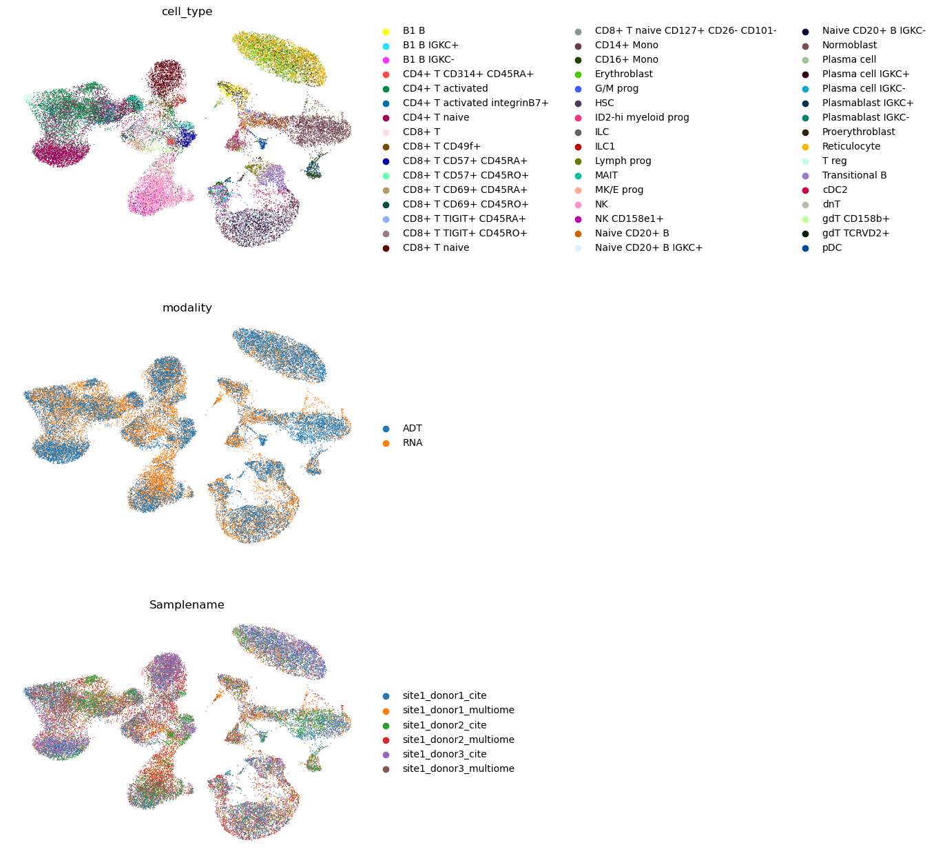
We see that the batches were well integrated as well as the two modalities. Yet again, scIB could be used to evaluate the integration.
45.5. Integration with partially overlapping data and query-to-reference mapping with totalVI#
Another multimodal data integration scenario is when we have paired and unpaired data available at the same time, for instance, a CITE-seq and an RNA-seq datasets. This scenario is also known as mosaic integration. We might be interested in mapping the datasets into a shared latent space to make use of all the data available to us. Another use case would be to impute missing modalities (i.e. proteins abundance for RNA-seq dataset). We show how to perform these two tasks, partially overlapping integration and imputation, using totalVI [Gayoso et al., 2021].
We set the protein counts of one of the batches to zeros to model the missing proteins. This helps later with mapping of the new RNA-only queries.
adata = rna_cite.copy()
adata.obsm["protein_counts"] = adt_cite.layers["counts"].A.copy()
adata.obsm["protein_counts"][adata.obs["batch"] == "s1d3"] = 0.0
adata
AnnData object with n_obs × n_vars = 16294 × 4000
    obs: 'GEX_n_genes_by_counts', 'GEX_pct_counts_mt', 'GEX_size_factors', 'GEX_phase', 'ADT_n_antibodies_by_counts', 'ADT_total_counts', 'ADT_iso_count', 'cell_type', 'batch', 'ADT_pseudotime_order', 'GEX_pseudotime_order', 'Samplename', 'Site', 'DonorNumber', 'Modality', 'VendorLot', 'DonorID', 'DonorAge', 'DonorBMI', 'DonorBloodType', 'DonorRace', 'Ethnicity', 'DonorGender', 'QCMeds', 'DonorSmoker', 'is_train', 'new_batch'
    var: 'feature_types', 'gene_id', 'highly_variable', 'means', 'dispersions', 'dispersions_norm'
    uns: 'dataset_id', 'genome', 'hvg', 'organism'
    obsm: 'ADT_X_pca', 'ADT_X_umap', 'ADT_isotype_controls', 'GEX_X_pca', 'GEX_X_umap', 'protein_counts'
    layers: 'counts'
Next, we setup the AnnData, specify the model parameters and train the model.
TOTALVI.setup_anndata(
    adata,
    layer="counts",
    batch_key="batch",
    protein_expression_obsm_key="protein_counts",
)
No GPU/TPU found, falling back to CPU. (Set TF_CPP_MIN_LOG_LEVEL=0 and rerun for more info.)
INFO     Generating sequential column names
INFO     Found batches with missing protein expression
arches_params = {
    "use_layer_norm": "both",
    "use_batch_norm": "none",
    "n_layers_decoder": 2,
    "n_layers_encoder": 2,
}

vae = TOTALVI(adata, **arches_params)
vae.train()
INFO Computing empirical prior initialization for protein background.
GPU available: True (cuda), used: True
TPU available: False, using: 0 TPU cores
IPU available: False, using: 0 IPUs
HPU available: False, using: 0 HPUs
LOCAL_RANK: 0 - CUDA_VISIBLE_DEVICES: [0]
Epoch 258/400:  64%|██████▍   | 258/400 [06:23<03:23,  1.43s/it, loss=709, v_num=1]Epoch 00258: reducing learning rate of group 0 to 2.4000e-03.
Epoch 381/400:  95%|█████████▌| 381/400 [09:23<00:27,  1.44s/it, loss=703, v_num=1]Epoch 00381: reducing learning rate of group 0 to 1.4400e-03.
Epoch 400/400: 100%|██████████| 400/400 [09:51<00:00,  1.44s/it, loss=710, v_num=1]
`Trainer.fit` stopped: `max_epochs=400` reached.
Epoch 400/400: 100%|██████████| 400/400 [09:51<00:00, 1.48s/it, loss=710, v_num=1]
Now we obtain the latent representation and visualize it.
adata.obsm["X_totalvi"] = vae.get_latent_representation()
sc.pp.neighbors(adata, use_rep="X_totalvi")
sc.tl.umap(adata)
sc.pl.umap(adata, color=["cell_type", "batch"], ncols=1, frameon=False)
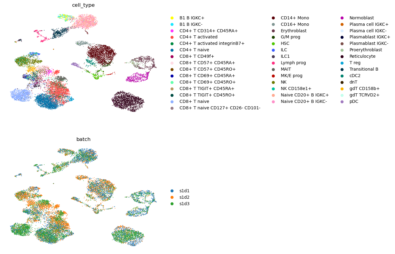
We see that batches as well as paired/RNA-only data are well integrated.
45.5.1. Query-to-reference mapping#
Now we demonstrate how to map new unimodal (RNA-only) and multimodal query (CITE-seq) onto the above reference.
We mimic RNA-only query by setting the protein counts of one of the two batches to zero.
query = rna_cite_query.copy()
query.obsm["protein_counts"] = adt_cite_query.layers["counts"].A.copy()
query.obsm["protein_counts"][query.obs["batch"] == "s2d4"] = 0.0
We create some additional columns in .obs to help with the visualization later.
adata.obs["dataset_name"] = "Reference"
query.obs["dataset_name"] = "Query"
adata.obs["dataset_name_fine"] = "CITE reference"
adata.obs["dataset_name_fine"][adata.obs["batch"] == "s1d3"] = "RNA reference"
query.obs["dataset_name_fine"] = "CITE query"
query.obs["dataset_name_fine"][query.obs["batch"] == "s2d4"] = "RNA query"
Next, we update and fine-tune the model.
vae_q = TOTALVI.load_query_data(
    query,
    vae,
)
vae_q.train(
    plan_kwargs={"weight_decay": 0.0, "scale_adversarial_loss": 0.0},
)
INFO     Found batches with missing protein expression
INFO     Computing empirical prior initialization for protein background.
GPU available: True (cuda), used: True
TPU available: False, using: 0 TPU cores
IPU available: False, using: 0 IPUs
HPU available: False, using: 0 HPUs
LOCAL_RANK: 0 - CUDA_VISIBLE_DEVICES: [0]
Epoch 233/400:  58%|█████▊    | 233/400 [05:32<03:54,  1.40s/it, loss=546, v_num=1]Epoch 00233: reducing learning rate of group 0 to 2.4000e-03.
Epoch 273/400:  68%|██████▊   | 273/400 [06:29<02:58,  1.40s/it, loss=548, v_num=1]Epoch 00273: reducing learning rate of group 0 to 1.4400e-03.
Epoch 287/400:  72%|███████▏  | 287/400 [06:49<02:41,  1.43s/it, loss=542, v_num=1]
Monitored metric elbo_validation did not improve in the last 45 records. Best score: 1102.225. Signaling Trainer to stop.
Finally, we obtain the latent representation for the query and visualize it together with the reference. For this we concatenate reference and the query and recalculate the neighbors and the UMAP.
query.obsm["X_totalvi_scarches"] = vae_q.get_latent_representation(query)
adata.obsm["X_totalvi_scarches"] = adata.obsm["X_totalvi"]
full_data = adata.concatenate(query, batch_key="concat_batch")
full_data
AnnData object with n_obs × n_vars = 32340 × 4000
    obs: 'GEX_n_genes_by_counts', 'GEX_pct_counts_mt', 'GEX_size_factors', 'GEX_phase', 'ADT_n_antibodies_by_counts', 'ADT_total_counts', 'ADT_iso_count', 'cell_type', 'batch', 'ADT_pseudotime_order', 'GEX_pseudotime_order', 'Samplename', 'Site', 'DonorNumber', 'Modality', 'VendorLot', 'DonorID', 'DonorAge', 'DonorBMI', 'DonorBloodType', 'DonorRace', 'Ethnicity', 'DonorGender', 'QCMeds', 'DonorSmoker', 'is_train', 'new_batch', '_scvi_labels', '_scvi_batch', 'dataset_name', 'dataset_name_fine', 'concat_batch'
    var: 'feature_types', 'gene_id', 'highly_variable', 'means', 'dispersions', 'dispersions_norm'
    obsm: 'ADT_X_pca', 'ADT_X_umap', 'ADT_isotype_controls', 'GEX_X_pca', 'GEX_X_umap', 'protein_counts', 'X_totalvi_scarches'
    layers: 'counts'
sc.pp.neighbors(full_data, use_rep="X_totalvi_scarches")
sc.tl.umap(full_data)
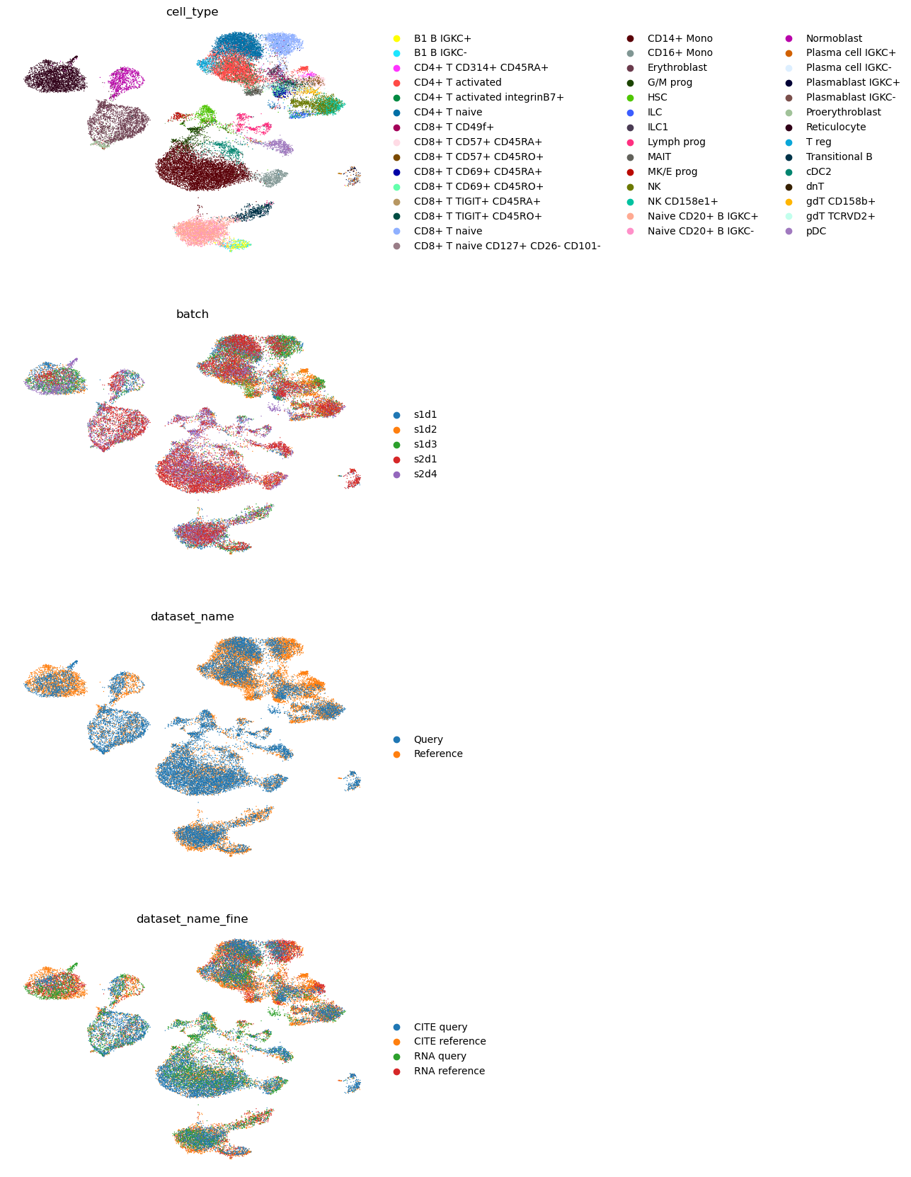
sc.pl.umap(
    full_data,
    color=["cell_type", "batch", "dataset_name", "dataset_name_fine"],
    ncols=1,
    frameon=False,
)
45.6. Query mapping and imputation with Seurat’s WNN#
Seurat v4 allows mapping of new RNA-seq queries onto a multimodal reference integrated with weighted-nearest-neighbor (WNN) [Hao et al., 2021]. We use the reference we built in the paired integration notebook.
The mapping is based on finding anchors between the query and the reference. This approach also allows for missing information transfer from the reference to the query. Here we show how to predict cell types and how to impute missing modalities (protein abundance in this case).
We note that since Seurat v4 is an R library we will need to work with anndata2ri package (theislab/anndata2ri) to move all of our data from Python to R.
First, let’s take a look at our reference and the query.
%%R
ref <- readRDS(cite, file = "wnn_ref.rds")
ref
An object of class Seurat
4136 features across 16294 samples within 2 assays
Active assay: RNA (4000 features, 4000 variable features)
 1 other assay present: ADT
 4 dimensional reductions calculated: pca, harmony_pca, spca, wnn.umap
rna_cite_query
AnnData object with n_obs × n_vars = 16046 × 4000
    obs: 'GEX_n_genes_by_counts', 'GEX_pct_counts_mt', 'GEX_size_factors', 'GEX_phase', 'ADT_n_antibodies_by_counts', 'ADT_total_counts', 'ADT_iso_count', 'cell_type', 'batch', 'ADT_pseudotime_order', 'GEX_pseudotime_order', 'Samplename', 'Site', 'DonorNumber', 'Modality', 'VendorLot', 'DonorID', 'DonorAge', 'DonorBMI', 'DonorBloodType', 'DonorRace', 'Ethnicity', 'DonorGender', 'QCMeds', 'DonorSmoker', 'is_train', 'new_batch'
    var: 'feature_types', 'gene_id', 'highly_variable', 'means', 'dispersions', 'dispersions_norm'
    uns: 'dataset_id', 'genome', 'hvg', 'organism'
    obsm: 'ADT_X_pca', 'ADT_X_umap', 'ADT_isotype_controls', 'GEX_X_pca', 'GEX_X_umap'
    layers: 'counts'
We need to preprocess the query first, so we use CLR-normalized counts to calculate PCA.
sc.pp.pca(rna_cite_query)
rna_cite_query
AnnData object with n_obs × n_vars = 16046 × 4000
    obs: 'GEX_n_genes_by_counts', 'GEX_pct_counts_mt', 'GEX_size_factors', 'GEX_phase', 'ADT_n_antibodies_by_counts', 'ADT_total_counts', 'ADT_iso_count', 'cell_type', 'batch', 'ADT_pseudotime_order', 'GEX_pseudotime_order', 'Samplename', 'Site', 'DonorNumber', 'Modality', 'VendorLot', 'DonorID', 'DonorAge', 'DonorBMI', 'DonorBloodType', 'DonorRace', 'Ethnicity', 'DonorGender', 'QCMeds', 'DonorSmoker', 'is_train', 'new_batch'
    var: 'feature_types', 'gene_id', 'highly_variable', 'means', 'dispersions', 'dispersions_norm'
    uns: 'dataset_id', 'genome', 'hvg', 'organism', 'pca'
    obsm: 'ADT_X_pca', 'ADT_X_umap', 'ADT_isotype_controls', 'GEX_X_pca', 'GEX_X_umap', 'X_pca'
    varm: 'PCs'
    layers: 'counts'
np.max(rna_cite_query.X)
9.061238
Next, we move the query from Python to R.
adata_ = sc.AnnData(rna_cite_query.X.copy())
adata_.obs_names = rna_cite_query.obs_names.copy()
adata_.var_names = rna_cite_query.var_names.copy()
adata_.obs["cell_type"] = rna_cite_query.obs["cell_type"].copy()
adata_.obs["batch"] = rna_cite_query.obs["batch"].copy()
adata_.obsm["X_pca"] = rna_cite_query.obsm["X_pca"].copy()
%%R -i adata_
query = as.Seurat(adata_, data='X', counts=NULL)
query
An object of class Seurat
4000 features across 16046 samples within 1 assay
Active assay: originalexp (4000 features, 0 variable features)
 1 dimensional reduction calculated: PCA
Now we need to find anchors between the reference and the query. We specify that we want to use SPCA dimensionality reduction from the reference.
%%R
anchors <- FindTransferAnchors(
  reference = ref,
  query = query,
  reference.reduction = "spca",
  dims = 1:20
)
Next, we map query onto the reference using the saved UMAP model to make sure that the UMAP projections stay the same for the reference and the query is mapped onto it. We additionally specify what information we want to transfer from the reference to the query with refdata parameter: in our case we want to predict the cell type and the protein counts.
%%R
query <- MapQuery(
  anchorset = anchors,
  query = query,
  reference = ref,
  refdata = list(
    cell_type = "cell_type",
    predicted_ADT = "ADT"
  ),
  reference.reduction = "spca",
  reduction.model = "wnn.umap",
  verbose=FALSE
)
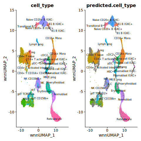
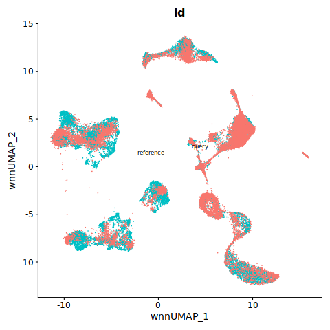
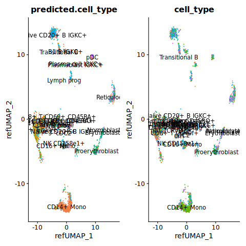
Let’s visualize the reference and the query together and take a look at predicted vs true cell labels.
%%R
ref$id <- 'reference'
query$id <- 'query'
refquery <-  merge(ref, query)
refquery[["umap"]] <- merge(ref[["wnn.umap"]], query[["ref.umap"]])
%%R
p1 <- DimPlot(refquery, reduction = "umap", group.by = "cell_type", label = TRUE, label.size = 3, repel = TRUE) + NoLegend()
p2 <- DimPlot(refquery, reduction = "umap", group.by = "predicted.cell_type", label = TRUE, label.size = 3, repel = TRUE) + NoLegend()
p1 + p2
Fontconfig warning: ignoring UTF-8: not a valid region tag
%%R
DimPlot(refquery, reduction = "umap", group.by = "id", label = TRUE, label.size = 3, repel = TRUE) + NoLegend()
45.7. Mapping ADT onto an RNA atlas with bridge integration#
Bridge [Hao et al., 2022] is a method for mapping new modalities onto an RNA-seq reference. To do so we need a so-called “bridge” dataset that contains paired data (RNA-seq and the new modality we want to map).
Since we want to showcase the bridging functionality, we assume that our reference consist of only one batch. We refer the reader to the integration vignette if there is a need to integrate batches in the reference (https://satijalab.org/seurat/articles/integration_introduction.html). As the bridge dataset we use one batch of the CITE-seq query, and as the actual ADT query we use ADT modality of the second batch in the CITE-seq query.
First, we subset the datasets to reference, bridge and query as described above.
rna_cite_ref = rna_cite[rna_cite.obs["batch"] == "s1d1"].copy()
rna_cite_bridge = rna_cite_query[rna_cite_query.obs["batch"] == "s2d1"].copy()
adt_cite_bridge = adt_cite_query[adt_cite_query.obs["donor"] == "s2d1"].copy()
adt_cite_query_bridge = adt_cite_query[adt_cite_query.obs["donor"] == "s2d4"].copy()
Next, we prepare the reference. We move the object from Python to R, normalize the data with SCTransform and calculate PCA. We also calculate the UMAP (and keep the model) that we will later use to map query onto.
adata_ = sc.AnnData(rna_cite_ref.layers["counts"].A.copy())
adata_.obs_names = rna_cite_ref.obs_names.copy()
adata_.var_names = rna_cite_ref.var_names.copy()
adata_.obs["cell_type"] = rna_cite_ref.obs["cell_type"].copy()
%%R -i adata_
ref = as.Seurat(adata_, data=NULL, counts='X')
ref
An object of class Seurat
4000 features across 5219 samples within 1 assay
Active assay: originalexp (4000 features, 0 variable features)
%%R
ref <- RenameAssays(object = ref, originalexp = "RNA", verbose=FALSE)
ref <- SCTransform(ref, verbose=FALSE)
ref <- RunPCA(ref, verbose=FALSE)
ref <- RunUMAP(ref, dims = 1:50, return.model=TRUE, verbose=FALSE)
Next, we prepare the bridge dataset. We move both RNA and ADT objects to R, follow the same normalization procedure as above for RNA, perform CLR-normalization and calculate PCA for ADT counts.
adata_ = sc.AnnData(adt_cite_bridge.layers["counts"].A.copy())
adata_.obs_names = adt_cite_bridge.obs_names.copy()
adata_.var_names = adt_cite_bridge.var_names.copy()
adata_.obs["cell_type"] = adt_cite_bridge.obs["cell_type"].copy()
adata_
AnnData object with n_obs × n_vars = 10465 × 136
    obs: 'cell_type'
%%R -i adata_
adt <- as.Seurat(adata_, data=NULL, counts='X')
adata_ = sc.AnnData(rna_cite_bridge.layers["counts"].A.copy())
adata_.obs_names = rna_cite_bridge.obs_names.copy()
adata_.var_names = rna_cite_bridge.var_names.copy()
adata_.obs["cell_type"] = rna_cite_bridge.obs["cell_type"].copy()
%%R -i adata_
rna = as.Seurat(adata_, data=NULL, counts='X')
cite <- rna
cite <- RenameAssays(object = cite, originalexp = "RNA")
cite[["ADT"]] <- CreateAssayObject(counts = adt@assays$originalexp@data)
%%R
DefaultAssay(cite) <- "RNA"
VariableFeatures(cite) <- rownames(cite)
cite <- SCTransform(cite, verbose = FALSE)
%%R
DefaultAssay(cite) <- "ADT"
VariableFeatures(cite) <- rownames(cite)
cite <- NormalizeData(cite, normalization.method = 'CLR', margin = 2, verbose=FALSE)
cite <- ScaleData(cite, verbose=FALSE)
Finally, we prepare the ADT query the same way as the bridge ADT above.
adata_ = sc.AnnData(adt_cite_query_bridge.layers["counts"].A.copy())
adata_.obs_names = adt_cite_query_bridge.obs_names.copy()
adata_.var_names = adt_cite_query_bridge.var_names.copy()
adata_.obs["cell_type"] = adt_cite_query_bridge.obs["cell_type"].copy()
%%R -i adata_
query <- as.Seurat(adata_, data=NULL, counts='X')
query <- RenameAssays(object = query, originalexp = "ADT", verbose=FALSE)
VariableFeatures(query) <- rownames(query)
query <- NormalizeData(query, normalization.method = 'CLR', margin = 2, verbose=FALSE)
query <- ScaleData(query, verbose=FALSE)
query <- RunPCA(query, verbose=FALSE, reduction.name = 'apca')
Now we can perform the bridge integration. The final step of query mapping is the same as with Seurat v4 query mapping so we can also predict cell types for the query data.
%%R
dims.adt <- 1:50
dims.rna <- 1:50

DefaultAssay(cite) <-  "RNA"
DefaultAssay(ref) <- "SCT"
obj.rna.ext <- PrepareBridgeReference(
    reference = ref,
    bridge = cite,
    bridge.query.assay = "ADT",
    reference.reduction = "pca",
    reference.dims = dims.rna,
    normalization.method = "SCT",
    verbose = FALSE
)
  |                                                  | 0 % ~calculating   |++++++++++++++++++++++++++++++++++++++++++++++++++| 100% elapsed=00s
  |                                                  | 0 % ~calculating   |++++++++++++++++++++++++++++++++++++++++++++++++++| 100% elapsed=00s
%%R
bridge.anchor <- FindBridgeTransferAnchors(
    extended.reference = obj.rna.ext,
    query = query,
    reduction = "pcaproject",
    dims = dims.adt,
    verbose = FALSE
)
| | 0 % ~calculating |++++++++++++++++++++++++++++++++++++++++++++++++++| 100% elapsed=00s
%%R
query <- MapQuery(
    anchorset = bridge.anchor,
    reference = ref,
    query = query,
    refdata = list(
        cell_type = "cell_type"
    ),
    reduction.model = "umap",
    verbose = FALSE
)
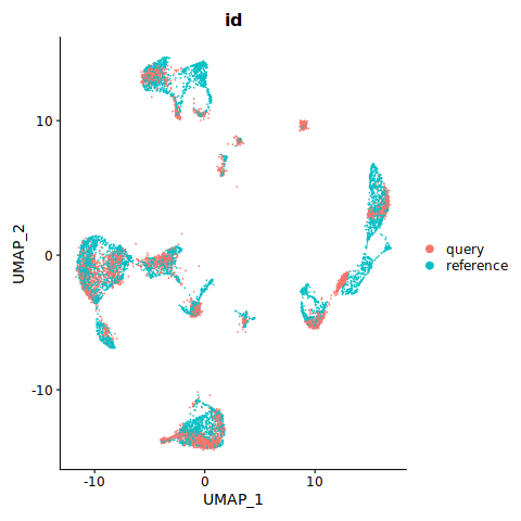
Let’s visualize the result.
%%R
p1 <- DimPlot(query, group.by = "predicted.cell_type", reduction = "ref.umap", label = TRUE) + NoLegend()
p2 <- DimPlot(query, group.by = "cell_type", reduction = "ref.umap", label = TRUE) + NoLegend()
p1 + p2
%%R
ref$id <- 'reference'
query$id <- 'query'
refquery <-  merge(ref, query)
refquery[["umap"]] <- merge(ref[["umap"]], query[["ref.umap"]])
DimPlot(refquery, group.by = 'id', shuffle = TRUE)
45.8. Trimodal integration and query-to-reference mapping with multigrate#
In our final example, we will build a trimodal reference atlas using RNA, ATAC and ADT as three modalities. Multigrate [Lotfollahi et al., 2022] is a deep-learning method based on conditional autoencoders. Data from each modality is fed into a separate encoder which outputs the parameters of the marginal distribution, then the parameters of the joint distribution are calculated with product of experts (PoE) [Lee and van der Schaar, 2021]. The conditional decoders then learn to reconstruct the original input data while simultaneously correction for batch effects. PoE allows the integration of data with missing measurements for some modalities by setting the corresponding marginals to a non-informative distribution. Multigrate also follows scArches [Lotfollahi et al., 2022] framework to allow query-to-reference mapping of unimodal as well as multimodal queries.
45.8.1. Building the reference#
First, we load data that has 4000 highly variable genes that are common for the scRNA-seq and scRNA-seq from the CITE-seq and the multiome experiment respectively.
rna1 = sc.read(
    "/lustre/groups/ml01/workspace/anastasia.litinetskaya/data/trimodal_neurips/rna_hvg_cite.h5ad"
)
rna1_ref = rna1[adt_cite.obs_names].copy()
rna1_query = rna1[adt_cite_query.obs_names].copy()
rna1_ref.shape, rna1_query.shape
((16294, 4000), (16046, 4000))
rna2 = sc.read(
    "/lustre/groups/ml01/workspace/anastasia.litinetskaya/data/trimodal_neurips/rna_hvg_multiome.h5ad"
)
rna2_ref = rna2[atac_multiome.obs_names].copy()
rna2_query = rna2[atac_multiome_query.obs_names].copy()
rna2_ref.shape, rna2_query.shape
((17243, 4000), (10331, 4000))
Next, we concatenate all the data into one AnnData object specifying how the data is paired and which layers to use.
adata = mtg.data.organize_multiome_anndatas(
    adatas=[[rna1_ref, rna2_ref], [None, atac_multiome], [adt_cite, None]],
    layers=[["counts", "counts"], [None, "cpm"], [None, None]],
)
adata
AnnData object with n_obs × n_vars = 33537 × 24136
    obs: 'GEX_n_genes_by_counts', 'GEX_pct_counts_mt', 'GEX_size_factors', 'GEX_phase', 'ADT_n_antibodies_by_counts', 'ADT_total_counts', 'ADT_iso_count', 'cell_type', 'batch', 'ADT_pseudotime_order', 'GEX_pseudotime_order', 'Samplename', 'Site', 'DonorNumber', 'Modality', 'VendorLot', 'DonorID', 'DonorAge', 'DonorBMI', 'DonorBloodType', 'DonorRace', 'Ethnicity', 'DonorGender', 'QCMeds', 'DonorSmoker', 'is_train', 'GEX_n_counts', 'GEX_n_genes', 'ATAC_nCount_peaks', 'ATAC_atac_fragments', 'ATAC_reads_in_peaks_frac', 'ATAC_blacklist_fraction', 'ATAC_nucleosome_signal', 'ATAC_pseudotime_order', 'technology', 'cell_type_l2', 'cell_type_l1', 'cell_type_l3', 'assay', 'split', 'group', 'balancing_weight', 'donor', 'log1p_n_genes_by_counts', 'log1p_total_counts', 'modality', 'n_counts', 'n_genes_by_counts', 'new_donor', 'outliers', 'total_counts', 'new_batch'
    var: 'modality'
    uns: 'modality_lengths'
    layers: 'counts'
Next, we register covariates that the model will correct for in the latent space.
mtg.model.MultiVAE.setup_anndata(
    adata,
    categorical_covariate_keys=["Modality", "Samplename"],
    rna_indices_end=4000,
)
Next, we initialize the model and train it.
model = mtg.model.MultiVAE(
    adata,
    losses=["nb", "mse", "mse"],
    loss_coefs={
        "kl": 1e-3,
        "integ": 10000,
    },
    integrate_on="Modality",
    mmd="marginal",
)
model.train()
GPU available: True (cuda), used: True
TPU available: False, using: 0 TPU cores
IPU available: False, using: 0 IPUs
HPU available: False, using: 0 HPUs
LOCAL_RANK: 0 - CUDA_VISIBLE_DEVICES: [0]
Epoch 200/200: 100%|██████████| 200/200 [28:53<00:00, 8.43s/it, loss=2.34e+03, v_num=1]
`Trainer.fit` stopped: `max_epochs=200` reached.
Epoch 200/200: 100%|██████████| 200/200 [28:53<00:00, 8.67s/it, loss=2.34e+03, v_num=1]
Finally, we obtain the latent representation, save it explicitly in .obsm['latent_ref'] as we will overwrite .obsm['latent'] later when we work with fine-tuned model after query mapping and visualize the result.
model.get_latent_representation()
adata.obsm["latent_ref"] = adata.obsm["latent"].copy()
adata
AnnData object with n_obs × n_vars = 33537 × 24136
    obs: 'GEX_n_genes_by_counts', 'GEX_pct_counts_mt', 'GEX_size_factors', 'GEX_phase', 'ADT_n_antibodies_by_counts', 'ADT_total_counts', 'ADT_iso_count', 'cell_type', 'batch', 'ADT_pseudotime_order', 'GEX_pseudotime_order', 'Samplename', 'Site', 'DonorNumber', 'Modality', 'VendorLot', 'DonorID', 'DonorAge', 'DonorBMI', 'DonorBloodType', 'DonorRace', 'Ethnicity', 'DonorGender', 'QCMeds', 'DonorSmoker', 'is_train', 'GEX_n_counts', 'GEX_n_genes', 'ATAC_nCount_peaks', 'ATAC_atac_fragments', 'ATAC_reads_in_peaks_frac', 'ATAC_blacklist_fraction', 'ATAC_nucleosome_signal', 'ATAC_pseudotime_order', 'technology', 'cell_type_l2', 'cell_type_l1', 'cell_type_l3', 'assay', 'split', 'group', 'balancing_weight', 'donor', 'log1p_n_genes_by_counts', 'log1p_total_counts', 'modality', 'n_counts', 'n_genes_by_counts', 'new_donor', 'outliers', 'total_counts', 'new_batch', 'size_factors', '_scvi_batch'
    var: 'modality'
    uns: 'modality_lengths', '_scvi_uuid', '_scvi_manager_uuid'
    obsm: '_scvi_extra_categorical_covs', 'latent', 'latent_ref'
    layers: 'counts'
sc.pp.neighbors(adata, use_rep="latent")
sc.tl.umap(adata)
sc.pl.umap(adata, color=["cell_type", "Modality", "Samplename"], ncols=1, frameon=False)
45.8.2. Querying the trimodal reference#
We repeat the same steps for the setting up the query as for the reference before.
query = mtg.data.organize_multiome_anndatas(
    adatas=[
        [rna1_query, rna2_query],
        [None, atac_multiome_query],
        [adt_cite_query, None],
    ],
    layers=[["counts", "counts"], [None, "cpm"], [None, None]],
)
mtg.model.MultiVAE.setup_anndata(
    query,
    categorical_covariate_keys=["Modality", "Samplename"],
    rna_indices_end=4000,
)
Let’s imitate unimodal queries by masking with zeros the snRNA part of one multiome batch and ADT part of one CITE-seq batch in the query. We get one ATAC-only query batch and one scRNA-only query batch respectively.
idx_atac_query = query.obs["Samplename"] == "site2_donor4_multiome"
idx_scrna_query = query.obs["Samplename"] == "site2_donor1_cite"

idx_mutiome_query = query.obs["Samplename"] == "site2_donor1_multiome"
idx_cite_query = query.obs["Samplename"] == "site2_donor4_cite"

(
    np.sum(idx_atac_query),
    np.sum(idx_scrna_query),
    np.sum(idx_mutiome_query),
    np.sum(idx_cite_query),
)
(6111, 10465, 4220, 5581)
query[idx_atac_query, :4000].X = 0
query[idx_scrna_query, 4000:].X = 0
We update the model by adding new weights to the new batches in the query and fine-tune those weights.
q_model = mtg.model.MultiVAE.load_query_data(query, model)
q_model.train(weight_decay=0)
GPU available: True (cuda), used: True
TPU available: False, using: 0 TPU cores
IPU available: False, using: 0 IPUs
HPU available: False, using: 0 HPUs
LOCAL_RANK: 0 - CUDA_VISIBLE_DEVICES: [0]
Epoch 200/200: 100%|██████████| 200/200 [16:13<00:00, 4.78s/it, loss=2.1e+03, v_num=1]
`Trainer.fit` stopped: `max_epochs=200` reached.
Epoch 200/200: 100%|██████████| 200/200 [16:13<00:00, 4.87s/it, loss=2.1e+03, v_num=1]
We obtain the latent representation for query and the reference from the updated model. Note that the representation of the reference is the same as before up to some sampling noise.
q_model.get_latent_representation(adata=query)
q_model.get_latent_representation(adata=adata)
INFO Input AnnData not setup with scvi-tools. attempting to transfer AnnData setup
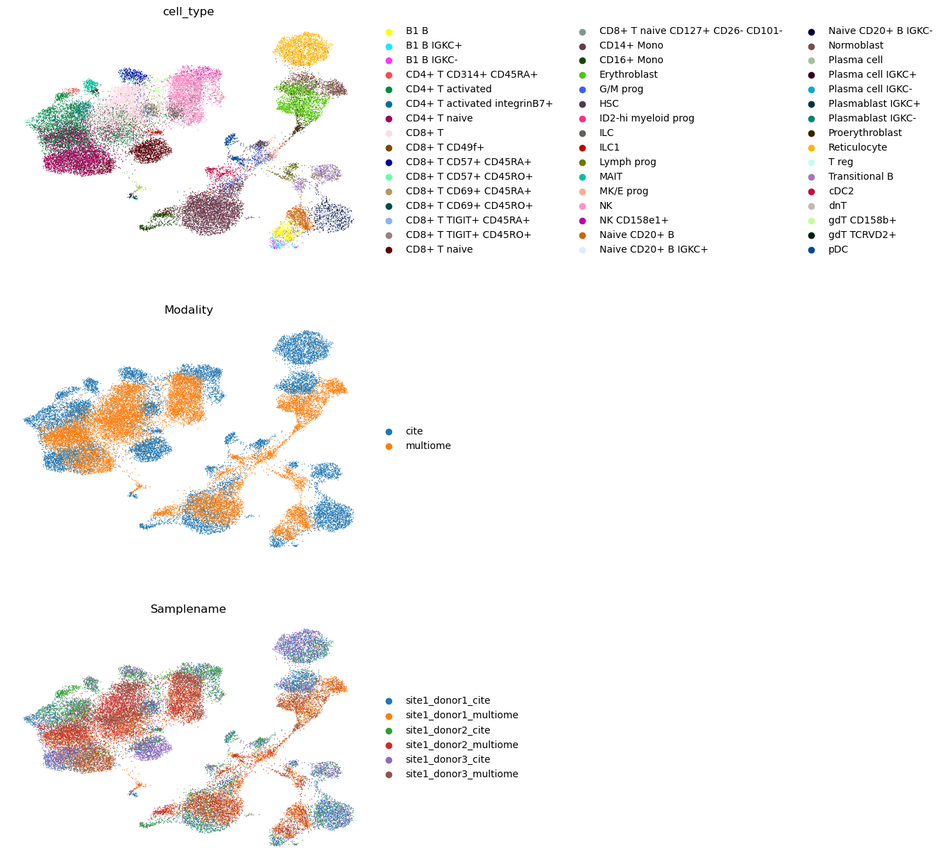
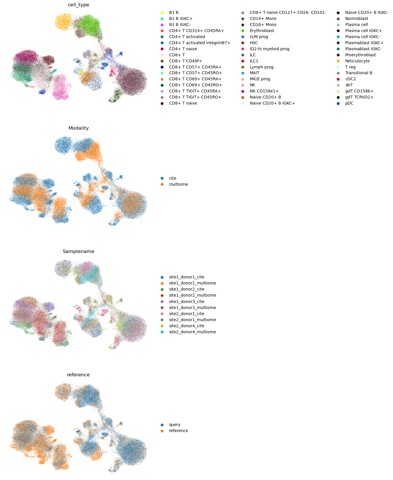
Finally, we concatenate the reference and the query, and visualize both on a UMAP.
adata.obs["reference"] = "reference"
query.obs["reference"] = "query"
adata.obs["type_of_query"] = "reference"
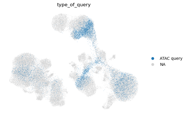
query.obs.loc[idx_atac_query, "type_of_query"] = "ATAC query"
query.obs.loc[idx_scrna_query, "type_of_query"] = "scRNA query"
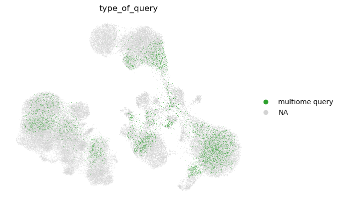
query.obs.loc[idx_mutiome_query, "type_of_query"] = "multiome query"
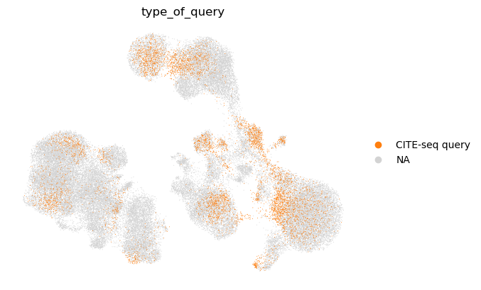
query.obs.loc[idx_cite_query, "type_of_query"] = "CITE-seq query"
adata_both = anndata.concat([adata, query])
sc.pp.neighbors(adata_both, use_rep="latent")
sc.tl.umap(adata_both)
sc.pl.umap(
    adata_both,
    color=["cell_type", "Modality", "Samplename", "reference"],
    ncols=1,
    frameon=False,
)
sc.pl.umap(
    adata_both, color="type_of_query", ncols=1, frameon=False, groups=["ATAC query"]
)
sc.pl.umap(
    adata_both, color="type_of_query", ncols=1, frameon=False, groups=["CITE-seq query"]
)
sc.pl.umap(
    adata_both, color="type_of_query", ncols=1, frameon=False, groups=["multiome query"]
)
sc.pl.umap(
    adata_both, color="type_of_query", ncols=1, frameon=False, groups=["scRNA query"]
)
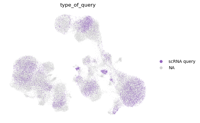
We observe that the query cell types are mapped to the corresponding cell types in the reference. We also note that unimodal query mapping is possible with Multigrate even though there was no unimodal data in the reference.
45.9. Session info#
%%R
sessionInfo()
R version 4.1.3 (2022-03-10)
Platform: x86_64-conda-linux-gnu (64-bit)
Running under: CentOS Linux 7 (Core)

Matrix products: default
BLAS/LAPACK: /lustre/groups/ml01/workspace/anastasia.litinetskaya/miniconda3/envs/advanced-integration/lib/libopenblasp-r0.3.21.so

locale:
 [1] LC_CTYPE=C                 LC_NUMERIC=C
 [3] LC_TIME=en_US.UTF-8        LC_COLLATE=en_US.UTF-8
 [5] LC_MONETARY=en_US.UTF-8    LC_MESSAGES=en_US.UTF-8
 [7] LC_PAPER=en_US.UTF-8       LC_NAME=C
 [9] LC_ADDRESS=C               LC_TELEPHONE=C
[11] LC_MEASUREMENT=en_US.UTF-8 LC_IDENTIFICATION=C

attached base packages:
[1] stats4    tools     stats     graphics  grDevices utils     datasets
[8] methods   base

other attached packages:
 [1] Matrix_1.5-3                SeuratObject_4.1.3
 [3] Seurat_4.1.1.9001           SingleCellExperiment_1.16.0
 [5] SummarizedExperiment_1.24.0 Biobase_2.54.0
 [7] GenomicRanges_1.46.1        GenomeInfoDb_1.30.1
 [9] IRanges_2.28.0              S4Vectors_0.32.4
[11] BiocGenerics_0.40.0         MatrixGenerics_1.6.0
[13] matrixStats_0.63.0

loaded via a namespace (and not attached):
  [1] Rtsne_0.16             colorspace_2.0-3       deldir_1.0-6
  [4] ellipsis_0.3.2         ggridges_0.5.4         XVector_0.34.0
  [7] RcppHNSW_0.4.1         spatstat.data_3.0-0    farver_2.1.1
 [10] leiden_0.4.3           listenv_0.9.0          ggrepel_0.9.2
 [13] RSpectra_0.16-1        fansi_1.0.3            codetools_0.2-18
 [16] splines_4.1.3          polyclip_1.10-4        jsonlite_1.8.4
 [19] ica_1.0-3              cluster_2.1.4          png_0.1-8
 [22] uwot_0.1.14            spatstat.sparse_3.0-0  shiny_1.7.4
 [25] sctransform_0.3.5      compiler_4.1.3         httr_1.4.4
 [28] fastmap_1.1.0          lazyeval_0.2.2         cli_3.5.0
 [31] later_1.3.0            htmltools_0.5.4        igraph_1.3.5
 [34] gtable_0.3.1           glue_1.6.2             GenomeInfoDbData_1.2.7
 [37] RANN_2.6.1             reshape2_1.4.4         dplyr_1.0.10
 [40] Rcpp_1.0.9             scattermore_0.8        vctrs_0.5.1
 [43] nlme_3.1-161           progressr_0.12.0       lmtest_0.9-40
 [46] spatstat.random_3.0-1  stringr_1.5.0          globals_0.16.2
 [49] mime_0.12              miniUI_0.1.1.1         lifecycle_1.0.3
 [52] irlba_2.3.5.1          goftest_1.2-3          future_1.30.0
 [55] zlibbioc_1.40.0        MASS_7.3-58.1          zoo_1.8-11
 [58] scales_1.2.1           spatstat.core_2.4-4    promises_1.2.0.1
 [61] spatstat.utils_3.0-1   parallel_4.1.3         RColorBrewer_1.1-3
 [64] reticulate_1.26        pbapply_1.6-0          gridExtra_2.3
 [67] ggplot2_3.4.0          rpart_4.1.19           stringi_1.7.8
 [70] fastDummies_1.6.3      rlang_1.0.6            pkgconfig_2.0.3
 [73] bitops_1.0-7           lattice_0.20-45        tensor_1.5
 [76] ROCR_1.0-11            purrr_1.0.0            labeling_0.4.2
 [79] patchwork_1.1.2        htmlwidgets_1.6.0      cowplot_1.1.1
 [82] tidyselect_1.2.0       parallelly_1.33.0      RcppAnnoy_0.0.20
 [85] plyr_1.8.8             magrittr_2.0.3         R6_2.5.1
 [88] generics_0.1.3         DelayedArray_0.20.0    withr_2.5.0
 [91] mgcv_1.8-41            pillar_1.8.1           fitdistrplus_1.1-8
 [94] abind_1.4-5            survival_3.4-0         RCurl_1.98-1.9
 [97] sp_1.5-1               tibble_3.1.8           future.apply_1.10.0
[100] crayon_1.5.2           KernSmooth_2.23-20     utf8_1.2.2
[103] spatstat.geom_3.0-3    plotly_4.10.1          grid_4.1.3
[106] data.table_1.14.6      digest_0.6.31          xtable_1.8-4
[109] tidyr_1.2.1            httpuv_1.6.7           munsell_0.5.0
[112] viridisLite_0.4.1
45.10. References#
Zhi-Jie Cao and Ge Gao. Multi-omics single-cell data integration and regulatory inference with graph-linked embedding. Nature Biotechnology, May 2022. URL: https://doi.org/10.1038/s41587-022-01284-4, doi:10.1038/s41587-022-01284-4.
Adam Gayoso, Zoë Steier, Romain Lopez, Jeffrey Regier, Kristopher L. Nazor, Aaron Streets, and Nir Yosef. Joint probabilistic modeling of single-cell multi-omic data with totalvi. Nature Methods, 18(3):272–282, Mar 2021. URL: https://doi.org/10.1038/s41592-020-01050-x, doi:10.1038/s41592-020-01050-x.
Yuhan Hao, Stephanie Hao, Erica Andersen-Nissen, William M. Mauck, Shiwei Zheng, Andrew Butler, Maddie J. Lee, Aaron J. Wilk, Charlotte Darby, Michael Zager, Paul Hoffman, Marlon Stoeckius, Efthymia Papalexi, Eleni P. Mimitou, Jaison Jain, Avi Srivastava, Tim Stuart, Lamar M. Fleming, Bertrand Yeung, Angela J. Rogers, Juliana M. McElrath, Catherine A. Blish, Raphael Gottardo, Peter Smibert, and Rahul Satija. Integrated analysis of multimodal single-cell data. Cell, 184(13):3573–3587.e29, 2021. URL: https://www.sciencedirect.com/science/article/pii/S0092867421005833, doi:https://doi.org/10.1016/j.cell.2021.04.048.
Yuhan Hao, Tim Stuart, Madeline Kowalski, Saket Choudhary, Paul Hoffman, Austin Hartman, Avi Srivastava, Gesmira Molla, Shaista Madad, Carlos Fernandez-Granda, and Rahul Satija. Dictionary learning for integrative, multimodal, and scalable single-cell analysis. bioRxiv, 2022. URL: https://www.biorxiv.org/content/early/2022/02/26/2022.02.24.481684, arXiv:https://www.biorxiv.org/content/early/2022/02/26/2022.02.24.481684.full.pdf, doi:10.1101/2022.02.24.481684.
Changhee Lee and Mihaela van der Schaar. A variational information bottleneck approach to multi-omics data integration. In Proceedings of The 24th International Conference on Artificial Intelligence and Statistics, volume 130 of Proceedings of Machine Learning Research, 1513–1521. 13–15 Apr 2021. URL: http://proceedings.mlr.press/v130/lee21a.html.
Mohammad Lotfollahi, Anastasia Litinetskaya, and Fabian J. Theis. Multigrate: single-cell multi-omic data integration. bioRxiv, 2022. URL: https://www.biorxiv.org/content/early/2022/03/17/2022.03.16.484643, arXiv:https://www.biorxiv.org/content/early/2022/03/17/2022.03.16.484643.full.pdf, doi:10.1101/2022.03.16.484643.
Mohammad Lotfollahi, Mohsen Naghipourfar, Malte D. Luecken, Matin Khajavi, Maren Büttner, Marco Wagenstetter, Žiga Avsec, Adam Gayoso, Nir Yosef, Marta Interlandi, Sergei Rybakov, Alexander V. Misharin, and Fabian J. Theis. Mapping single-cell data to reference atlases by transfer learning. Nature Biotechnology, 40(1):121–130, Jan 2022. URL: https://doi.org/10.1038/s41587-021-01001-7, doi:10.1038/s41587-021-01001-7.
Malte D Luecken, Daniel Bernard Burkhardt, Robrecht Cannoodt, Christopher Lance, Aditi Agrawal, Hananeh Aliee, Ann T Chen, Louise Deconinck, Angela M Detweiler, Alejandro A Granados, Shelly Huynh, Laura Isacco, Yang Joon Kim, Dominik Klein, BONY DE KUMAR, Sunil Kuppasani, Heiko Lickert, Aaron McGeever, Honey Mekonen, Joaquin Caceres Melgarejo, Maurizio Morri, Michaela Müller, Norma Neff, Sheryl Paul, Bastian Rieck, Kaylie Schneider, Scott Steelman, Michael Sterr, Daniel J. Treacy, Alexander Tong, Alexandra-Chloe Villani, Guilin Wang, Jia Yan, Ce Zhang, Angela Oliveira Pisco, Smita Krishnaswamy, Fabian J Theis, and Jonathan M. Bloom. A sandbox for prediction and integration of dna, rna, and proteins in single cells. In Thirty-fifth Conference on Neural Information Processing Systems Datasets and Benchmarks Track (Round 2). 2021. URL: https://openreview.net/forum?id=gN35BGa1Rt.
45.11. Contributors#
We gratefully acknowledge the contributions of:
45.11.2. Reviewers#
Lukas Heumos